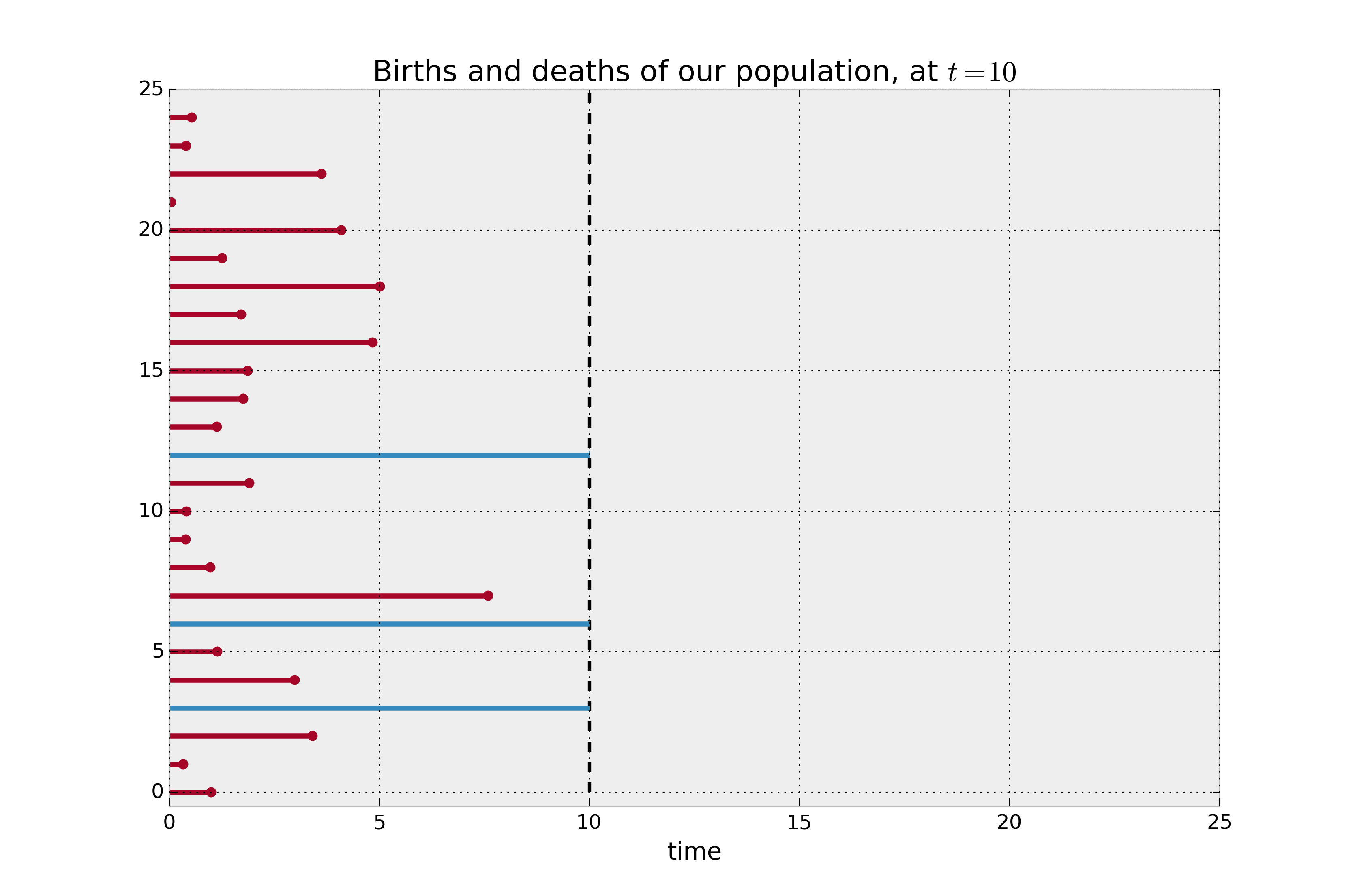
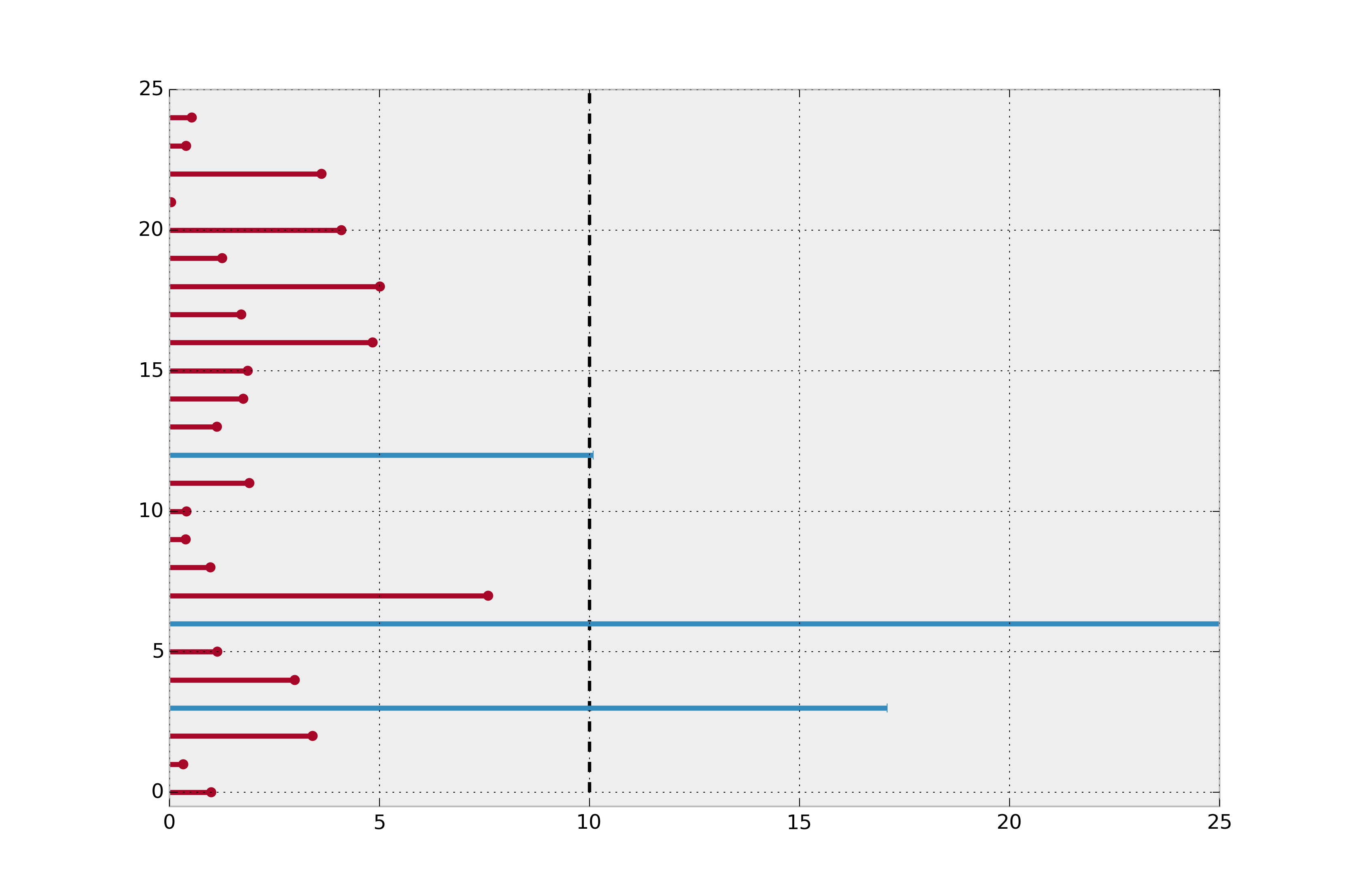
All we know is that actual lifetime is greater than some threshold. Mathematically, we know $P(T \ge t) = 1 - F(t) := S(t)$. We can use this in our log likelihood:
No censoring cases:
$$l(\theta, t) = \sum_{\text{observed}} \log{\text{pdf}(\theta, t)} $$With censoring cases: $$ \begin{align} l(\theta, t) & = \sum_{\text{observed}} \log{\text{pdf}(t, \theta)} + \sum_{\text{censored}} \log{\text{S}(t, \theta)} \\ & = \sum_{\text{observed}} \log{\text{pdf}(t, \theta)} \frac{S(t)}{S(t)} + \sum_{\text{censored}} \log{\text{S}(t, \theta)} \\ & = \sum_{\text{observed}} (\log{\frac{\text{pdf}(t, \theta)}{S(t)}} + \log{S(t)}) + \sum_{\text{censored}} \log{\text{S}(t, \theta)} \\ & = \sum_{\text{observed}} \log{\frac{\text{pdf}(t, \theta)}{S(t)}} + \sum_{\text{observed}} \log{S(t)} + \sum_{\text{censored}} \log{\text{S}(t, \theta)} \\ & = \sum_{\text{observed}} \log{\frac{\text{pdf}(t, \theta)}{S(t)}} + \sum \log{S(t)} \end{align} $$
The $-\log{S(t)}$ is known as the cumulative hazard, denoted $H(t)$.
$$l(\theta, t) = \sum_{\text{observed}} \log{\frac{\text{pdf}(t, \theta)}{S(t)}} - \sum H(t, \theta) $$Also, $\frac{dH}{dt} = \frac{\text{pdf}(t, \theta)}{S(t)}$. Denote that $h(t)$.
$$l(\theta, t) = \sum_{\text{observed}} \log{h(t, \theta}) - \sum H(t, \theta) $$Phew! Now, instead of working in probability space, we will work in hazard space! Here's a link to all the relatioships: https://lifelines.readthedocs.io/en/latest/Survival%20Analysis%20intro.html#hazard-function
Take away: the likelihood function can be used to "add" information about the system (think about how penalizers are used...)
# the hazard and cumulative hazard for Weibull are much simplier to implement 😗👌

def cumulative_hazard(params, t):
    lambda_, rho_ = params
    return (t / lambda_) ** rho_

def hazard(params, t):
    # diff of cumulative hazard w.r.t. t
    lambda_, rho_ = params
    return rho_ / lambda_ * (t / lambda_) ** (rho_ - 1)

def log_hazard(params, t):
    return np.log(hazard(params, t))

def log_likelihood(params, t, e):
    return np.sum(e * log_hazard(params, t)) - np.sum(cumulative_hazard(params, t))
T = (np.random.exponential(size=1000)/1.5) ** 2.3
E = np.random.binomial(1, 0.95, size=1000)

from scipy.optimize import minimize

results = minimize(log_likelihood,
        x0 = np.array([1.0, 1.0]),
        method=None,
        args=(T, E),
        bounds=((0.00001, None), (0.00001, None)))

print(results)
# why did this fail? Note the -inf.
def negative_log_likelihood(params, t, e):
    return -log_likelihood(params, t, e)

results = minimize( # what goes here?,
        x0 = np.array([1.0, 1.0]),
        method=None,
        args=(T, E),
        bounds=((0.00001, None), (0.00001, None)))

print(results)
t = np.linspace(0, 10, 100)
plt.plot(t, np.exp(-cumulative_hazard(results.x, t)))
plt.ylim(0, 1)
plt.title("Estimated survival function")
Let's move to part 3 - automatic differentiation!

