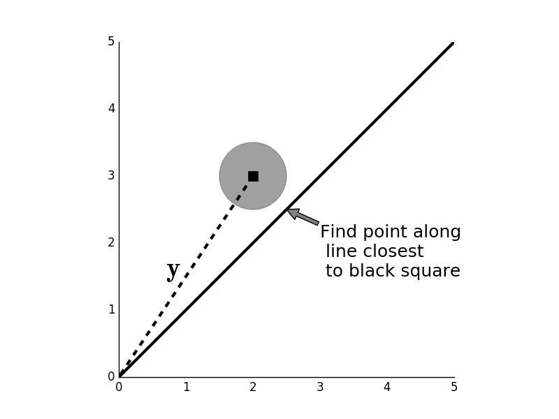
Given the point $\mathbf{y}$ (black # square) we want to find the $\mathbf{x}$ along the line that is closest to it. # The gray circle is the locus of points within a fixed distance from # $\mathbf{y}$.
# #
#
#
# **Programming Tip.**
#
# [Figure](#fig:probability_001) uses
# the `matplotlib.patches` module. This
# module contains primitive shapes like
# circles, ellipses, and rectangles that
# can be assembled into complex graphics.
# After importing a particular shape, you
# can apply that shape to an existing axis
# using the `add_patch` method. The
# patches themselves can by styled using the
# usual formatting keywords like
# `color` and `alpha`.
#
#
#
#
#
#
#
#
#
#
#
# **Programming Tip.**
#
# [Figure](#fig:probability_001) uses
# the `matplotlib.patches` module. This
# module contains primitive shapes like
# circles, ellipses, and rectangles that
# can be assembled into complex graphics.
# After importing a particular shape, you
# can apply that shape to an existing axis
# using the `add_patch` method. The
# patches themselves can by styled using the
# usual formatting keywords like
# `color` and `alpha`.
#
#
#
#
#
#
#
# The closest point on the line occurs when # the line is tangent to the circle. When this happens, the black line and the # line (minimum distance) are perpedicular.
# #
#
#
#
# Now that we
# can see what's going on, we can construct the the solution
# analytically. We can
# represent an arbitrary point along the black line as:
#
# $$
# \mathbf{x}=\alpha\mathbf{v}
# $$
#
# where $\alpha\in\mathbb{R}$ slides the point up and down the line with
#
# $$
# \mathbf{v} = \left[ 1,1 \right]^T
# $$
#
# Formally, $\mathbf{v}$ is the *subspace* onto which we want to
# *project*
# $\mathbf{y}$. At the closest point, the vector between
# $\mathbf{y}$ and
# $\mathbf{x}$ (the *error* vector above) is
# perpedicular to the line. This means
# that
#
# $$
# (\mathbf{y}-\mathbf{x} )^T \mathbf{v} = 0
# $$
#
# and by substituting and working out the terms, we obtain
#
# $$
# \alpha = \frac{\mathbf{y}^T\mathbf{v}}{ \|\mathbf{v} \|^2}
# $$
#
# The *error* is the distance between $\alpha\mathbf{v}$ and $
# \mathbf{y}$. This
# is a right triangle, and we can use the Pythagorean
# theorem to compute the
# squared length of this error as
#
# $$
# \epsilon^2 = \|( \mathbf{y}-\mathbf{x} )\|^2 = \|\mathbf{y}\|^2 - \alpha^2
# \|\mathbf{v}\|^2 = \|\mathbf{y}\|^2 -
# \frac{\|\mathbf{y}^T\mathbf{v}\|^2}{\|\mathbf{v}\|^2}
# $$
#
# where $ \|\mathbf{v}\|^2 = \mathbf{v}^T \mathbf{v} $. Note that since
# $\epsilon^2 \ge 0 $, this also shows that
#
# $$
# \| \mathbf{y}^T\mathbf{v}\| \le \|\mathbf{y}\| \|\mathbf{v}\|
# $$
#
# which is the famous and useful Cauchy-Schwarz inequality which we
# will exploit
# later. Finally, we can assemble all of this into the *projection*
# operator
#
# $$
# \mathbf{P}_v = \frac{1}{\|\mathbf{v}\|^2 } \mathbf{v v}^T
# $$
#
# With this operator, we can take any $\mathbf{y}$ and find the closest
# point on
# $\mathbf{v}$ by doing
#
# $$
# \mathbf{P}_v \mathbf{y} = \mathbf{v} \left( \frac{ \mathbf{v}^T \mathbf{y}
# }{\|\mathbf{v}\|^2} \right)
# $$
#
# where we recognize the term in parenthesis as the $\alpha$ we
# computed earlier.
# It's called an *operator* because it takes a vector
# ($\mathbf{y}$) and produces
# another vector ($\alpha\mathbf{v}$). Thus,
# projection unifies geometry and
# optimization.
#
# ## Weighted distance
#
# We can easily extend this projection
# operator to cases where the measure of
# distance between $\mathbf{y}$ and the
# subspace $\mathbf{v}$ is weighted. We can
# accommodate these weighted distances
# by re-writing the projection operator as
#
#
#
#
# $$
# \begin{equation}
# \mathbf{P}_v=\mathbf{v}\frac{\mathbf{v}^T\mathbf{Q}^T}{\mathbf{v}^T\mathbf{Q v}}
# \end{equation}
# \label{eq:weightedProj} \tag{1}
# $$
#
# where $\mathbf{Q}$ is positive definite matrix. In the previous
# case, we
# started with a point $\mathbf{y}$ and inflated a circle centered at
# $\mathbf{y}$
# until it just touched the line defined by $\mathbf{v}$ and this
# point was
# closest point on the line to $\mathbf{y}$. The same thing happens
# in the general
# case with a weighted distance except now we inflate an
# ellipse, not a circle,
# until the ellipse touches the line.
#
#
#
#
#
#
#
#
#
#
#
#
# Now that we
# can see what's going on, we can construct the the solution
# analytically. We can
# represent an arbitrary point along the black line as:
#
# $$
# \mathbf{x}=\alpha\mathbf{v}
# $$
#
# where $\alpha\in\mathbb{R}$ slides the point up and down the line with
#
# $$
# \mathbf{v} = \left[ 1,1 \right]^T
# $$
#
# Formally, $\mathbf{v}$ is the *subspace* onto which we want to
# *project*
# $\mathbf{y}$. At the closest point, the vector between
# $\mathbf{y}$ and
# $\mathbf{x}$ (the *error* vector above) is
# perpedicular to the line. This means
# that
#
# $$
# (\mathbf{y}-\mathbf{x} )^T \mathbf{v} = 0
# $$
#
# and by substituting and working out the terms, we obtain
#
# $$
# \alpha = \frac{\mathbf{y}^T\mathbf{v}}{ \|\mathbf{v} \|^2}
# $$
#
# The *error* is the distance between $\alpha\mathbf{v}$ and $
# \mathbf{y}$. This
# is a right triangle, and we can use the Pythagorean
# theorem to compute the
# squared length of this error as
#
# $$
# \epsilon^2 = \|( \mathbf{y}-\mathbf{x} )\|^2 = \|\mathbf{y}\|^2 - \alpha^2
# \|\mathbf{v}\|^2 = \|\mathbf{y}\|^2 -
# \frac{\|\mathbf{y}^T\mathbf{v}\|^2}{\|\mathbf{v}\|^2}
# $$
#
# where $ \|\mathbf{v}\|^2 = \mathbf{v}^T \mathbf{v} $. Note that since
# $\epsilon^2 \ge 0 $, this also shows that
#
# $$
# \| \mathbf{y}^T\mathbf{v}\| \le \|\mathbf{y}\| \|\mathbf{v}\|
# $$
#
# which is the famous and useful Cauchy-Schwarz inequality which we
# will exploit
# later. Finally, we can assemble all of this into the *projection*
# operator
#
# $$
# \mathbf{P}_v = \frac{1}{\|\mathbf{v}\|^2 } \mathbf{v v}^T
# $$
#
# With this operator, we can take any $\mathbf{y}$ and find the closest
# point on
# $\mathbf{v}$ by doing
#
# $$
# \mathbf{P}_v \mathbf{y} = \mathbf{v} \left( \frac{ \mathbf{v}^T \mathbf{y}
# }{\|\mathbf{v}\|^2} \right)
# $$
#
# where we recognize the term in parenthesis as the $\alpha$ we
# computed earlier.
# It's called an *operator* because it takes a vector
# ($\mathbf{y}$) and produces
# another vector ($\alpha\mathbf{v}$). Thus,
# projection unifies geometry and
# optimization.
#
# ## Weighted distance
#
# We can easily extend this projection
# operator to cases where the measure of
# distance between $\mathbf{y}$ and the
# subspace $\mathbf{v}$ is weighted. We can
# accommodate these weighted distances
# by re-writing the projection operator as
#
#
#
#
# $$
# \begin{equation}
# \mathbf{P}_v=\mathbf{v}\frac{\mathbf{v}^T\mathbf{Q}^T}{\mathbf{v}^T\mathbf{Q v}}
# \end{equation}
# \label{eq:weightedProj} \tag{1}
# $$
#
# where $\mathbf{Q}$ is positive definite matrix. In the previous
# case, we
# started with a point $\mathbf{y}$ and inflated a circle centered at
# $\mathbf{y}$
# until it just touched the line defined by $\mathbf{v}$ and this
# point was
# closest point on the line to $\mathbf{y}$. The same thing happens
# in the general
# case with a weighted distance except now we inflate an
# ellipse, not a circle,
# until the ellipse touches the line.
#
#
#
#
#
#
#
# In the weighted # case, the closest point on the line is tangent to the ellipse and is still # perpedicular in the sense of the weighted distance.
# #
#
#
#
# Note that the
# error vector ($\mathbf{y}-\alpha\mathbf{v}$) in [Figure](#fig:probability_003)
# is still perpendicular to the line (subspace
# $\mathbf{v}$), but in the space of
# the weighted distance. The difference
# between the first projection (with the
# uniform circular distance) and the
# general case (with the elliptical weighted
# distance) is the inner product
# between the two cases. For example, in the first
# case we have $\mathbf{y}^T
# \mathbf{v}$ and in the weighted case we have
# $\mathbf{y}^T \mathbf{Q}^T
# \mathbf{v}$. To move from the uniform circular case
# to the weighted ellipsoidal
# case, all we had to do was change all of the vector
# inner products. Before we
# finish, we need a formal property of projections:
#
# $$
# \mathbf{P}_v \mathbf{P}_v = \mathbf{P}_v
# $$
#
# known as the *idempotent* property which basically says that once we
# have
# projected onto a subspace, subsequent projections leave us in the
# same subspace.
# You can verify this by computing Equation [1](#eq:weightedProj).
#
# Thus,
# projection ties a minimization problem (closest point to a line) to an
# algebraic
# concept (inner product). It turns out that these same geometric ideas
# from
# linear algebra [[strang2006linear]](#strang2006linear) can be translated to the
# conditional
# expectation. How this works is the subject of our next section.
#
#
#
#
# Note that the
# error vector ($\mathbf{y}-\alpha\mathbf{v}$) in [Figure](#fig:probability_003)
# is still perpendicular to the line (subspace
# $\mathbf{v}$), but in the space of
# the weighted distance. The difference
# between the first projection (with the
# uniform circular distance) and the
# general case (with the elliptical weighted
# distance) is the inner product
# between the two cases. For example, in the first
# case we have $\mathbf{y}^T
# \mathbf{v}$ and in the weighted case we have
# $\mathbf{y}^T \mathbf{Q}^T
# \mathbf{v}$. To move from the uniform circular case
# to the weighted ellipsoidal
# case, all we had to do was change all of the vector
# inner products. Before we
# finish, we need a formal property of projections:
#
# $$
# \mathbf{P}_v \mathbf{P}_v = \mathbf{P}_v
# $$
#
# known as the *idempotent* property which basically says that once we
# have
# projected onto a subspace, subsequent projections leave us in the
# same subspace.
# You can verify this by computing Equation [1](#eq:weightedProj).
#
# Thus,
# projection ties a minimization problem (closest point to a line) to an
# algebraic
# concept (inner product). It turns out that these same geometric ideas
# from
# linear algebra [[strang2006linear]](#strang2006linear) can be translated to the
# conditional
# expectation. How this works is the subject of our next section.