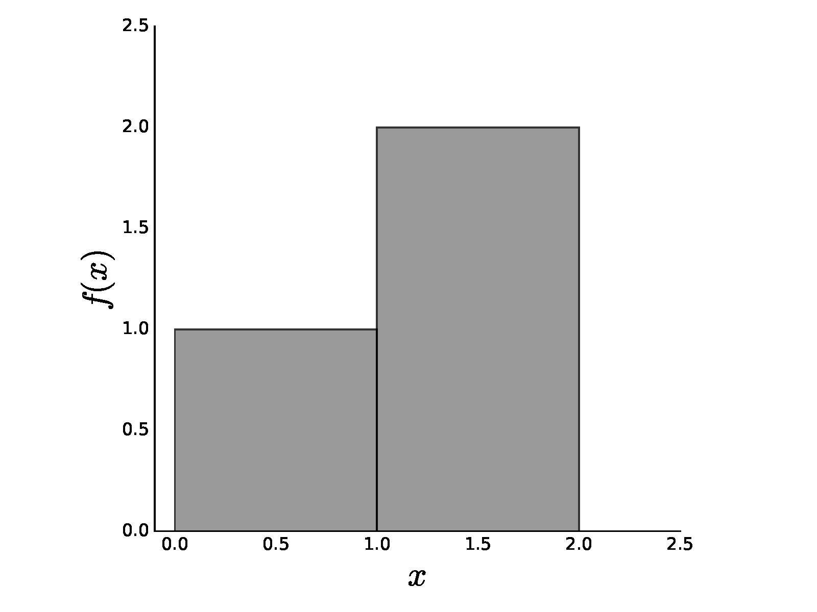
Simple piecewise-constant function.
# #
#
#
# $$
# \int_0^2 f(x) dx = 1 + 2 = 3
# $$
#
# which has the usual interpretation as the area of the two rectangles
# that make
# up $f(x)$. So far, so good.
#
# With Lesbesgue integration, the idea is very
# similar except that we
# focus on the y-axis instead of moving along the x-axis.
# The question
# is given $f(x) = 1$, what is the set of $x$ values for which this
# is
# true? For our example, this is true whenever $x\in (0,1]$. So now we
# have a
# correspondence between the values of the function (namely, `1`
# and `2`) and the
# sets of $x$ values for which this is true, namely,
# $\lbrace (0,1] \rbrace$ and
# $\lbrace (1,2] \rbrace$, respectively. To
# compute the integral, we simply take
# the function values (i.e., `1,2`)
# and some way of measuring the size of the
# corresponding interval
# (i.e., $\mu$) as in the following:
#
# $$
# \int_0^2 f d\mu = 1 \mu(\lbrace (0,1] \rbrace) + 2 \mu(\lbrace (1,2] \rbrace)
# $$
#
# We have suppressed some of the notation above to emphasize generality. Note
# that
# we obtain the same value of the integral as in the Riemann case when
# $\mu((0,1])
# = \mu((1,2]) = 1$. By introducing the $\mu$ function as a way of
# measuring the
# intervals above, we have introduced another degree of freedom in
# our
# integration. This accommodates many weird functions that are not tractable
# using
# the usual Riemann theory, but we refer you to a proper introduction to
# Lesbesgue
# integration for further study [[jones2001lebesgue]](#jones2001lebesgue).
# Nonetheless,
# the key step in the above discussion is the introduction of the
# $\mu$ function,
# which we will encounter again as the so-called probability
# density function.
#
# ## Random Variables
#
# Most introductions to probability jump
# straight into *random variables* and
# then explain how to compute complicated
# integrals. The problem with this
# approach is that it skips over some of the
# important subtleties that we will now
# consider. Unfortunately, the term *random
# variable* is not very descriptive. A
# better term is *measurable function*. To
# understand why this is a better term,
# we have to dive into the formal
# constructions of probability by way of a simple
# example.
#
# Consider tossing a
# fair six-sided die. There are only six outcomes possible,
#
# $$
# \Omega=\lbrace 1,2,3,4,5,6 \rbrace
# $$
#
# As we know, if the die is fair, then the probability of each outcome is $1/6$.
# To say this formally, the measure of each set (i.e., $\lbrace 1 \rbrace,\lbrace
# 2 \rbrace,\ldots,\lbrace 6 \rbrace$) is $\mu(\lbrace 1 \rbrace ) =\mu(\lbrace 2
# \rbrace ) \ldots = \mu(\lbrace 6 \rbrace ) = 1/6$. In this case, the $\mu$
# function we discussed earlier is the usual *probability* mass function, denoted
# by
# $\mathbb{P}$. The measurable function maps a set into a
# number on the real
# line. For example, $ \lbrace 1 \rbrace \mapsto 1 $ is
# one such function.
#
# Now,
# here's where things get interesting. Suppose you were asked to construct a
# fair
# coin from the fair die. In other words, we want to throw the die and then
# record
# the outcomes as if we had just tossed a fair coin. How could we do this?
# One way
# would be to define a measurable function that says if the die comes up
# `3` or
# less, then we declare *heads* and otherwise declare *tails*. This has
# some
# strong intuition behind it, but let's articulate it in terms of formal
# theory.
# This strategy creates two different non-overlapping sets $\lbrace
# 1,2,3 \rbrace$
# and $\lbrace 4,5,6 \rbrace$. Each set has the same probability
# *measure*,
#
# $$
# \begin{eqnarray*}
# \mathbb{P}(\lbrace 1,2,3 \rbrace) & = & 1/2 \\\
# \mathbb{P}(\lbrace 4,5,6 \rbrace) & = & 1/2
# \end{eqnarray*}
# $$
#
# And the problem is solved. Everytime the die comes up
# $\lbrace 1,2,3 \rbrace$,
# we record heads and record tails otherwise.
#
# Is this the only way to construct a
# fair coin experiment from a
# fair die? Alternatively, we can define the sets as
# $\lbrace 1 \rbrace$,
# $\lbrace 2 \rbrace$, $\lbrace 3,4,5,6 \rbrace$. If we
# define the corresponding
# measure for each set as the following
#
# $$
# \begin{eqnarray*}
# \mathbb{P}(\lbrace 1 \rbrace) & = & 1/2 \\\
# \mathbb{P}(\lbrace 2 \rbrace) & = & 1/2 \\\
# \mathbb{P}(\lbrace 3,4,5,6 \rbrace)
# & = & 0
# \end{eqnarray*}
# $$
#
# then, we have another solution to the fair coin problem. To
# implement this,
# all we do is ignore every time the die shows `3,4,5,6` and
# throw again. This is
# wasteful, but it solves the problem. Nonetheless,
# we hope you can see how the
# interlocking pieces of the theory provide a
# framework for carrying the notion of
# uncertainty/potentiality from one problem
# to the next (e.g., from the fair die
# to the fair coin).
#
# Let's consider a slightly more interesting problem where we
# toss two dice. We
# assume that each throw is *independent*, meaning that the
# outcome of one does
# not influence the other. What are the sets in this case?
# They are all pairs
# of possible outcomes from two throws as shown below,
#
# $$
# \Omega = \lbrace (1,1),(1,2),\ldots,(5,6),(6,6) \rbrace
# $$
#
# What are the measures of each of these sets? By virtue of the
# independence
# claim, the measure of each is the product of the respective measures
# of each
# element. For instance,
#
# $$
# \mathbb{P}((1,2)) = \mathbb{P}(\lbrace 1 \rbrace) \mathbb{P}(\lbrace 2
# \rbrace) = \frac{1}{6^2}
# $$
#
# With all that established, we can ask the following
# question: what is the
# probability that the sum of the dice equals
# seven? As before, the first thing to
# do is characterize the
# measurable function for this as $X:(a,b) \mapsto (a+b)$.
# Next, we
# associate all of the $(a,b)$ pairs with their sum. We can create a
# Python dictionary for this as shown,
# In[2]:
d={(i,j):i+j for i in range(1,7) for j in range(1,7)}
# The next step is to collect all of the $(a,b)$ pairs that sum to
# each of the
# possible values from two to twelve.
# In[3]:
from collections import defaultdict
dinv = defaultdict(list)
for i,j in d.items():
dinv[j].append(i)
# **Programming Tip.**
#
# The `defaultdict` object from the built-in collections
# module creates dictionaries with
# default values when it encounters a new key.
# Otherwise, we would have had to
# create default values manually for a regular
# dictionary.
#
#
#
# For example, `dinv[7]` contains the following list of pairs that
# sum to seven,
# In[4]:
dinv[7]
# The next step is to compute the probability measured for each of these items.
# Using the independence assumption, this means we have to compute the sum of the
# products of the individual item probabilities in `dinv`. Because we know that
# each outcome is equally likely, the probability of every term in the sum equals
# $1/36$. Thus, all
# we have to do is count the number of items in the
# corresponding list for each
# key in `dinv` and divide by `36`. For example,
# `dinv[11]` contains `[(5, 6),
# (6, 5)]`. The probability of `5+6=6+5=11` is the
# probability of this set which
# is composed of the sum of the probabilities of the
# individual elements
# `{(5,6),(6,5)}`. In this case, we have $\mathbb{P}(11) =
# \mathbb{P}(\lbrace
# (5,6) \rbrace)+ \mathbb{P}(\lbrace (6,5) \rbrace) = 1/36 +
# 1/36 = 2/36$.
# Repeating this procedure for all the elements, we derive the
# probability mass
# function as shown below,
# In[5]:
X={i:len(j)/36. for i,j in dinv.items()}
print(X)
# **Programming Tip.**
#
# In the preceding code note that `36.` is written with
# the
# trailing decimal mark. This is a good habit to get into
# because the default
# division operation changed between Python 2.x and
# Python 3.x. In Python 2.x
# division is integer division by default,
# and it is floating-point division in
# Python 3.x.
#
#
#
# The above example exposes the elements of probability theory that
# are in play for this simple problem while deliberately suppressing some of the
# gory technical details. With this framework, we can ask other questions like
# what is the probability that half the product of three dice will exceed the
# their sum? We can solve this using the same method as in the following. First,
# let's create the first mapping,
# In[6]:
d={(i,j,k):((i*j*k)/2>i+j+k) for i in range(1,7)
for j in range(1,7)
for k in range(1,7)}
# The keys of this dictionary are the triples and the values are the
# logical
# values of whether or not half the product of three dice exceeds their sum.
# Now,
# we do the inverse mapping to collect the corresponding lists,
# In[7]:
dinv = defaultdict(list)
for i,j in d.items():
dinv[j].append(i)
# Note that `dinv` contains only two keys, `True` and `False`. Again,
# because the
# dice are independent, the probability of any triple is $1/6^3$.
# Finally, we
# collect this for each outcome as in the following,
# In[8]:
X={i:len(j)/6.0**3 for i,j in dinv.items()}
print(X)
# Thus, the probability of half the product of three dice exceeding their sum is
# `136/(6.0**3) = 0.63`. The set that is induced by the random variable has only
# two elements in it, `True` and `False`, with $\mathbb{P}(\mbox{True})=136/216$
# and $\mathbb{P}(\mbox{False})=1-136/216$.
#
# As a final example to exercise
# another layer of generality, let is consider the
# first problem with the two dice
# where we want the probability of a
# seven, but this time one of the dice is no
# longer fair. The distribution for
# the unfair die is the following:
#
# $$
# \begin{eqnarray*}
# \mathbb{P}(\lbrace 1\rbrace)=\mathbb{P}(\lbrace 2
# \rbrace)=\mathbb{P}(\lbrace 3 \rbrace) = \frac{1}{9} \\\
# \mathbb{P}(\lbrace
# 4\rbrace)=\mathbb{P}(\lbrace 5 \rbrace)=\mathbb{P}(\lbrace 6 \rbrace) =
# \frac{2}{9}
# \end{eqnarray*}
# $$
#
# From our earlier work, we know the elements corresponding to the sum of seven
# are the following:
#
# $$
# \lbrace (1,6),(2,5),(3,4),(4,3),(5,2),(6,1) \rbrace
# $$
#
# Because we still have the independence assumption, all we need to
# change is
# the probability computation of each of elements. For example, given
# that the
# first die is the unfair one, we have
#
# $$
# \mathbb{P}((1,6)) = \mathbb{P}(1)\mathbb{P}(6) = \frac{1}{9} \times
# \frac{1}{6}
# $$
#
# and likewise for $(2,5)$ we have the following:
#
# $$
# \mathbb{P}((2,5)) = \mathbb{P}(2)\mathbb{P}(5) = \frac{1}{9} \times
# \frac{1}{6}
# $$
#
# and so forth. Summing all of these gives the following:
#
# $$
# \mathbb{P}_X(7) = \frac{1}{9} \times \frac{1}{6}
# +\frac{1}{9} \times \frac{1}{6}
# +\frac{1}{9} \times
# \frac{1}{6}
# +\frac{2}{9} \times \frac{1}{6}
# +\frac{2}{9} \times \frac{1}{6}
# +\frac{2}{9} \times
# \frac{1}{6} = \frac{1}{6}
# $$
#
# Let's try computing this using Pandas instead
# of Python dictionaries. First, we
# construct
# a `DataFrame` object with an index of tuples
# consisting of all pairs
# of possible dice outcomes.
# In[9]:
from pandas import DataFrame
d=DataFrame(index=[(i,j) for i in range(1,7) for j in range(1,7)],
columns=['sm','d1','d2','pd1','pd2','p'])
# Now, we can populate the columns that we set up above
# where the outcome of the
# first die is the `d1` column and
# the outcome of the second die is `d2`,
# In[10]:
d.d1=[i[0] for i in d.index]
d.d2=[i[1] for i in d.index]
# Next, we compute the sum of the dices in the `sm`
# column,
# In[11]:
d.sm=list(map(sum,d.index))
# With that established, the DataFrame now looks like
# the following:
# In[12]:
d.head(5) # show first five lines
# Next, we fill out the probabilities for each face of the
# unfair die (`d1`) and
# the fair die (`d2`),
# In[13]:
d.loc[d.d1<=3,'pd1']=1/9.
d.loc[d.d1 > 3,'pd1']=2/9.
d.pd2=1/6.
d.head(10)
# Finally, we can compute the joint probabilities
# for the sum of the shown faces
# as the following:
# In[14]:
d.p = d.pd1 * d.pd2
d.head(5)
# With all that established, we can compute the
# density of all the dice outcomes
# by using `groupby` as in the
# following,
# In[15]:
d.groupby('sm')['p'].sum()
# These examples have shown how the theory of probability
# breaks down sets and
# measurements of those sets and how these can be
# combined to develop the
# probability mass functions for new random
# variables.
#
# ## Continuous Random
# Variables
#
# The same ideas work with continuous variables but managing the sets
# becomes trickier because the real line, unlike discrete sets, has many
# limiting
# properties already built into it that have to be handled
# carefully.
# Nonetheless, let's start with an example that should
# illustrate the analogous
# ideas. Suppose a random variable $X$ is
# uniformly distributed on the unit
# interval. What is the probability
# that the variable takes on values less than
# 1/2?
#
# In order to build intuition onto the discrete case, let's go back to our
# dice-throwing experiment with the fair dice. The sum of the values of the dice
# is a measurable function,
#
# $$
# Y \colon \lbrace 1,2,\dots,6 \rbrace^2 \mapsto \lbrace 2,3,\ldots, 12 \rbrace
# $$
#
# That is, $Y$ is a mapping of the cartesian product of sets to a
# discrete set of
# outcomes. In order to compute probabilities of the set of
# outcomes, we need to
# derive the probability measure for $Y$, $\mathbb{P}_Y$,
# from the corresponding
# probability measures for each die. Our previous discussion
# went through the
# mechanics of that. This means that
#
# $$
# \mathbb{P}_Y \colon \lbrace 2,3,\ldots,12 \rbrace \mapsto [0,1]
# $$
#
# Note there is a separation between the function definition and where the
# target
# items of the function are measured in probability. More bluntly,
#
# $$
# Y \colon A \mapsto B
# $$
#
# with,
#
# $$
# \mathbb{P}_Y \colon B \mapsto [0,1]
# $$
#
# Thus, to compute $\mathbb{P}_Y$, which is derived
# from other random variables,
# we have to express the equivalence classes
# in $B$ in terms of their progenitor
# $A$ sets.
#
# The situation for continuous variables follows the same pattern, but
# with many more deep technicalities that we are going to skip. For the continuous
# case, the random variable is now,
#
# $$
# X \colon \mathbb{R} \mapsto \mathbb{R}
# $$
#
# with corresponding probability measure,
#
# $$
# \mathbb{P}_X \colon \mathbb{R} \mapsto [0,1]
# $$
#
# But where are the corresponding sets here? Technically, these are the
# *Borel*
# sets, but we can just think of them as intervals. Returning to our
# question,
# what is the probability that a uniformly distributed random variable
# on the unit
# interval takes values less than $1/2$? Rephrasing this question
# according to the
# framework, we have the following:
#
# $$
# X \colon [0,1] \mapsto [0,1]
# $$
#
# with corresponding,
#
# $$
# \mathbb{P}_X \colon [0,1] \mapsto [0,1]
# $$
#
# To answer the question, by the definition of the uniform random
# variable on
# the unit interval, we compute the following integral,
#
# $$
# \mathbb{P}_X([0,1/2]) = \mathbb{P}_X(0 < X < 1/2) = \int_0^{1/2} dx = 1/2
# $$
#
# where the above integral's $dx$ sweeps through intervals of the
# $B$-type. The
# measure of any $dx$ interval (i.e., $A$-type set) is equal to
# $dx$, by
# definition of the uniform random variable. To get all the moving parts
# into one
# notationally rich integral, we can also write this as,
#
# $$
# \mathbb{P}_X(0 < X < 1/2) = \int_0^{ 1/2 } d\mathbb{P}_X(dx) = 1/2
# $$
#
# Now, let's consider a slightly more complicated and interesting example. As
# before, suppose we have a uniform random variable, $X$ and let us introduce
# another random variable defined,
#
# $$
# Y = 2 X
# $$
#
# Now, what is the probability that $0 < Y < \frac{1}{2}$?
# To express this in
# our framework, we write,
#
# $$
# Y \colon [0,1] \mapsto [0,2]
# $$
#
# with corresponding,
#
# $$
# \mathbb{P}_Y \colon [0,2] \mapsto [0,1]
# $$
#
# To answer the question, we need to measure the set $[0,1/2]$, with
# the
# probability measure for $Y$, $\mathbb{P}_Y([0,1/2])$. How can we do this?
# Because $Y$ is derived from the $X$ random variable, as with the fair-dice
# throwing experiment, we have to create a set of equivalences in the target
# space
# (i.e., $B$-type sets) that reflect back on the input space (i.e.,
# $A$-type
# sets). That is, what is the interval $[0,1/2]$ equivalent to in terms
# of the $X$
# random variable? Because, functionally, $Y=2 X$, then the $B$-type
# interval
# $[0,1/2]$ corresponds to the $A$-type interval $[0,1/4]$. From the
# probability
# measure of $X$, we compute this with the integral,
#
# $$
# \mathbb{P}_Y([0,1/2]) =\mathbb{P}_X([0,1/4])= \int_0^{1/4} dx = 1/4
# $$
#
# Now, let's up the ante and consider the following random variable,
#
# $$
# Y = X^2
# $$
#
# where now $X$ is still uniformly distributed, but now over the
# interval
# $[-1/2,1/2]$. We can express this in our framework as,
#
# $$
# Y \colon [-1/2,1/2] \mapsto [0,1/4]
# $$
#
# with corresponding,
#
# $$
# \mathbb{P}_Y \colon [0,1/4] \mapsto [0,1]
# $$
#
# What is the $\mathbb{P}_Y(Y < 1/8)$? In other words, what is the
# measure of
# the set $B_Y= [0,1/8]$? As before, because $X$ is derived from our
# uniformly
# distributed random variable, we have to reflect the $B_Y$ set onto
# sets of the
# $A$-type. The thing to recognize is that because $X^2$
# is symmetric about zero,
# all $B_Y$ sets reflect back into two sets.
# This means that for any set $B_Y$, we
# have the correspondence $B_Y = A_X^+ \cup
# A_X^{-}$. So, we have,
#
# $$
# B_Y=\Big\lbrace 0
#
#
#
# $$
# \int_0^2 f(x) dx = 1 + 2 = 3
# $$
#
# which has the usual interpretation as the area of the two rectangles
# that make
# up $f(x)$. So far, so good.
#
# With Lesbesgue integration, the idea is very
# similar except that we
# focus on the y-axis instead of moving along the x-axis.
# The question
# is given $f(x) = 1$, what is the set of $x$ values for which this
# is
# true? For our example, this is true whenever $x\in (0,1]$. So now we
# have a
# correspondence between the values of the function (namely, `1`
# and `2`) and the
# sets of $x$ values for which this is true, namely,
# $\lbrace (0,1] \rbrace$ and
# $\lbrace (1,2] \rbrace$, respectively. To
# compute the integral, we simply take
# the function values (i.e., `1,2`)
# and some way of measuring the size of the
# corresponding interval
# (i.e., $\mu$) as in the following:
#
# $$
# \int_0^2 f d\mu = 1 \mu(\lbrace (0,1] \rbrace) + 2 \mu(\lbrace (1,2] \rbrace)
# $$
#
# We have suppressed some of the notation above to emphasize generality. Note
# that
# we obtain the same value of the integral as in the Riemann case when
# $\mu((0,1])
# = \mu((1,2]) = 1$. By introducing the $\mu$ function as a way of
# measuring the
# intervals above, we have introduced another degree of freedom in
# our
# integration. This accommodates many weird functions that are not tractable
# using
# the usual Riemann theory, but we refer you to a proper introduction to
# Lesbesgue
# integration for further study [[jones2001lebesgue]](#jones2001lebesgue).
# Nonetheless,
# the key step in the above discussion is the introduction of the
# $\mu$ function,
# which we will encounter again as the so-called probability
# density function.
#
# ## Random Variables
#
# Most introductions to probability jump
# straight into *random variables* and
# then explain how to compute complicated
# integrals. The problem with this
# approach is that it skips over some of the
# important subtleties that we will now
# consider. Unfortunately, the term *random
# variable* is not very descriptive. A
# better term is *measurable function*. To
# understand why this is a better term,
# we have to dive into the formal
# constructions of probability by way of a simple
# example.
#
# Consider tossing a
# fair six-sided die. There are only six outcomes possible,
#
# $$
# \Omega=\lbrace 1,2,3,4,5,6 \rbrace
# $$
#
# As we know, if the die is fair, then the probability of each outcome is $1/6$.
# To say this formally, the measure of each set (i.e., $\lbrace 1 \rbrace,\lbrace
# 2 \rbrace,\ldots,\lbrace 6 \rbrace$) is $\mu(\lbrace 1 \rbrace ) =\mu(\lbrace 2
# \rbrace ) \ldots = \mu(\lbrace 6 \rbrace ) = 1/6$. In this case, the $\mu$
# function we discussed earlier is the usual *probability* mass function, denoted
# by
# $\mathbb{P}$. The measurable function maps a set into a
# number on the real
# line. For example, $ \lbrace 1 \rbrace \mapsto 1 $ is
# one such function.
#
# Now,
# here's where things get interesting. Suppose you were asked to construct a
# fair
# coin from the fair die. In other words, we want to throw the die and then
# record
# the outcomes as if we had just tossed a fair coin. How could we do this?
# One way
# would be to define a measurable function that says if the die comes up
# `3` or
# less, then we declare *heads* and otherwise declare *tails*. This has
# some
# strong intuition behind it, but let's articulate it in terms of formal
# theory.
# This strategy creates two different non-overlapping sets $\lbrace
# 1,2,3 \rbrace$
# and $\lbrace 4,5,6 \rbrace$. Each set has the same probability
# *measure*,
#
# $$
# \begin{eqnarray*}
# \mathbb{P}(\lbrace 1,2,3 \rbrace) & = & 1/2 \\\
# \mathbb{P}(\lbrace 4,5,6 \rbrace) & = & 1/2
# \end{eqnarray*}
# $$
#
# And the problem is solved. Everytime the die comes up
# $\lbrace 1,2,3 \rbrace$,
# we record heads and record tails otherwise.
#
# Is this the only way to construct a
# fair coin experiment from a
# fair die? Alternatively, we can define the sets as
# $\lbrace 1 \rbrace$,
# $\lbrace 2 \rbrace$, $\lbrace 3,4,5,6 \rbrace$. If we
# define the corresponding
# measure for each set as the following
#
# $$
# \begin{eqnarray*}
# \mathbb{P}(\lbrace 1 \rbrace) & = & 1/2 \\\
# \mathbb{P}(\lbrace 2 \rbrace) & = & 1/2 \\\
# \mathbb{P}(\lbrace 3,4,5,6 \rbrace)
# & = & 0
# \end{eqnarray*}
# $$
#
# then, we have another solution to the fair coin problem. To
# implement this,
# all we do is ignore every time the die shows `3,4,5,6` and
# throw again. This is
# wasteful, but it solves the problem. Nonetheless,
# we hope you can see how the
# interlocking pieces of the theory provide a
# framework for carrying the notion of
# uncertainty/potentiality from one problem
# to the next (e.g., from the fair die
# to the fair coin).
#
# Let's consider a slightly more interesting problem where we
# toss two dice. We
# assume that each throw is *independent*, meaning that the
# outcome of one does
# not influence the other. What are the sets in this case?
# They are all pairs
# of possible outcomes from two throws as shown below,
#
# $$
# \Omega = \lbrace (1,1),(1,2),\ldots,(5,6),(6,6) \rbrace
# $$
#
# What are the measures of each of these sets? By virtue of the
# independence
# claim, the measure of each is the product of the respective measures
# of each
# element. For instance,
#
# $$
# \mathbb{P}((1,2)) = \mathbb{P}(\lbrace 1 \rbrace) \mathbb{P}(\lbrace 2
# \rbrace) = \frac{1}{6^2}
# $$
#
# With all that established, we can ask the following
# question: what is the
# probability that the sum of the dice equals
# seven? As before, the first thing to
# do is characterize the
# measurable function for this as $X:(a,b) \mapsto (a+b)$.
# Next, we
# associate all of the $(a,b)$ pairs with their sum. We can create a
# Python dictionary for this as shown,
# In[2]:
d={(i,j):i+j for i in range(1,7) for j in range(1,7)}
# The next step is to collect all of the $(a,b)$ pairs that sum to
# each of the
# possible values from two to twelve.
# In[3]:
from collections import defaultdict
dinv = defaultdict(list)
for i,j in d.items():
dinv[j].append(i)
# **Programming Tip.**
#
# The `defaultdict` object from the built-in collections
# module creates dictionaries with
# default values when it encounters a new key.
# Otherwise, we would have had to
# create default values manually for a regular
# dictionary.
#
#
#
# For example, `dinv[7]` contains the following list of pairs that
# sum to seven,
# In[4]:
dinv[7]
# The next step is to compute the probability measured for each of these items.
# Using the independence assumption, this means we have to compute the sum of the
# products of the individual item probabilities in `dinv`. Because we know that
# each outcome is equally likely, the probability of every term in the sum equals
# $1/36$. Thus, all
# we have to do is count the number of items in the
# corresponding list for each
# key in `dinv` and divide by `36`. For example,
# `dinv[11]` contains `[(5, 6),
# (6, 5)]`. The probability of `5+6=6+5=11` is the
# probability of this set which
# is composed of the sum of the probabilities of the
# individual elements
# `{(5,6),(6,5)}`. In this case, we have $\mathbb{P}(11) =
# \mathbb{P}(\lbrace
# (5,6) \rbrace)+ \mathbb{P}(\lbrace (6,5) \rbrace) = 1/36 +
# 1/36 = 2/36$.
# Repeating this procedure for all the elements, we derive the
# probability mass
# function as shown below,
# In[5]:
X={i:len(j)/36. for i,j in dinv.items()}
print(X)
# **Programming Tip.**
#
# In the preceding code note that `36.` is written with
# the
# trailing decimal mark. This is a good habit to get into
# because the default
# division operation changed between Python 2.x and
# Python 3.x. In Python 2.x
# division is integer division by default,
# and it is floating-point division in
# Python 3.x.
#
#
#
# The above example exposes the elements of probability theory that
# are in play for this simple problem while deliberately suppressing some of the
# gory technical details. With this framework, we can ask other questions like
# what is the probability that half the product of three dice will exceed the
# their sum? We can solve this using the same method as in the following. First,
# let's create the first mapping,
# In[6]:
d={(i,j,k):((i*j*k)/2>i+j+k) for i in range(1,7)
for j in range(1,7)
for k in range(1,7)}
# The keys of this dictionary are the triples and the values are the
# logical
# values of whether or not half the product of three dice exceeds their sum.
# Now,
# we do the inverse mapping to collect the corresponding lists,
# In[7]:
dinv = defaultdict(list)
for i,j in d.items():
dinv[j].append(i)
# Note that `dinv` contains only two keys, `True` and `False`. Again,
# because the
# dice are independent, the probability of any triple is $1/6^3$.
# Finally, we
# collect this for each outcome as in the following,
# In[8]:
X={i:len(j)/6.0**3 for i,j in dinv.items()}
print(X)
# Thus, the probability of half the product of three dice exceeding their sum is
# `136/(6.0**3) = 0.63`. The set that is induced by the random variable has only
# two elements in it, `True` and `False`, with $\mathbb{P}(\mbox{True})=136/216$
# and $\mathbb{P}(\mbox{False})=1-136/216$.
#
# As a final example to exercise
# another layer of generality, let is consider the
# first problem with the two dice
# where we want the probability of a
# seven, but this time one of the dice is no
# longer fair. The distribution for
# the unfair die is the following:
#
# $$
# \begin{eqnarray*}
# \mathbb{P}(\lbrace 1\rbrace)=\mathbb{P}(\lbrace 2
# \rbrace)=\mathbb{P}(\lbrace 3 \rbrace) = \frac{1}{9} \\\
# \mathbb{P}(\lbrace
# 4\rbrace)=\mathbb{P}(\lbrace 5 \rbrace)=\mathbb{P}(\lbrace 6 \rbrace) =
# \frac{2}{9}
# \end{eqnarray*}
# $$
#
# From our earlier work, we know the elements corresponding to the sum of seven
# are the following:
#
# $$
# \lbrace (1,6),(2,5),(3,4),(4,3),(5,2),(6,1) \rbrace
# $$
#
# Because we still have the independence assumption, all we need to
# change is
# the probability computation of each of elements. For example, given
# that the
# first die is the unfair one, we have
#
# $$
# \mathbb{P}((1,6)) = \mathbb{P}(1)\mathbb{P}(6) = \frac{1}{9} \times
# \frac{1}{6}
# $$
#
# and likewise for $(2,5)$ we have the following:
#
# $$
# \mathbb{P}((2,5)) = \mathbb{P}(2)\mathbb{P}(5) = \frac{1}{9} \times
# \frac{1}{6}
# $$
#
# and so forth. Summing all of these gives the following:
#
# $$
# \mathbb{P}_X(7) = \frac{1}{9} \times \frac{1}{6}
# +\frac{1}{9} \times \frac{1}{6}
# +\frac{1}{9} \times
# \frac{1}{6}
# +\frac{2}{9} \times \frac{1}{6}
# +\frac{2}{9} \times \frac{1}{6}
# +\frac{2}{9} \times
# \frac{1}{6} = \frac{1}{6}
# $$
#
# Let's try computing this using Pandas instead
# of Python dictionaries. First, we
# construct
# a `DataFrame` object with an index of tuples
# consisting of all pairs
# of possible dice outcomes.
# In[9]:
from pandas import DataFrame
d=DataFrame(index=[(i,j) for i in range(1,7) for j in range(1,7)],
columns=['sm','d1','d2','pd1','pd2','p'])
# Now, we can populate the columns that we set up above
# where the outcome of the
# first die is the `d1` column and
# the outcome of the second die is `d2`,
# In[10]:
d.d1=[i[0] for i in d.index]
d.d2=[i[1] for i in d.index]
# Next, we compute the sum of the dices in the `sm`
# column,
# In[11]:
d.sm=list(map(sum,d.index))
# With that established, the DataFrame now looks like
# the following:
# In[12]:
d.head(5) # show first five lines
# Next, we fill out the probabilities for each face of the
# unfair die (`d1`) and
# the fair die (`d2`),
# In[13]:
d.loc[d.d1<=3,'pd1']=1/9.
d.loc[d.d1 > 3,'pd1']=2/9.
d.pd2=1/6.
d.head(10)
# Finally, we can compute the joint probabilities
# for the sum of the shown faces
# as the following:
# In[14]:
d.p = d.pd1 * d.pd2
d.head(5)
# With all that established, we can compute the
# density of all the dice outcomes
# by using `groupby` as in the
# following,
# In[15]:
d.groupby('sm')['p'].sum()
# These examples have shown how the theory of probability
# breaks down sets and
# measurements of those sets and how these can be
# combined to develop the
# probability mass functions for new random
# variables.
#
# ## Continuous Random
# Variables
#
# The same ideas work with continuous variables but managing the sets
# becomes trickier because the real line, unlike discrete sets, has many
# limiting
# properties already built into it that have to be handled
# carefully.
# Nonetheless, let's start with an example that should
# illustrate the analogous
# ideas. Suppose a random variable $X$ is
# uniformly distributed on the unit
# interval. What is the probability
# that the variable takes on values less than
# 1/2?
#
# In order to build intuition onto the discrete case, let's go back to our
# dice-throwing experiment with the fair dice. The sum of the values of the dice
# is a measurable function,
#
# $$
# Y \colon \lbrace 1,2,\dots,6 \rbrace^2 \mapsto \lbrace 2,3,\ldots, 12 \rbrace
# $$
#
# That is, $Y$ is a mapping of the cartesian product of sets to a
# discrete set of
# outcomes. In order to compute probabilities of the set of
# outcomes, we need to
# derive the probability measure for $Y$, $\mathbb{P}_Y$,
# from the corresponding
# probability measures for each die. Our previous discussion
# went through the
# mechanics of that. This means that
#
# $$
# \mathbb{P}_Y \colon \lbrace 2,3,\ldots,12 \rbrace \mapsto [0,1]
# $$
#
# Note there is a separation between the function definition and where the
# target
# items of the function are measured in probability. More bluntly,
#
# $$
# Y \colon A \mapsto B
# $$
#
# with,
#
# $$
# \mathbb{P}_Y \colon B \mapsto [0,1]
# $$
#
# Thus, to compute $\mathbb{P}_Y$, which is derived
# from other random variables,
# we have to express the equivalence classes
# in $B$ in terms of their progenitor
# $A$ sets.
#
# The situation for continuous variables follows the same pattern, but
# with many more deep technicalities that we are going to skip. For the continuous
# case, the random variable is now,
#
# $$
# X \colon \mathbb{R} \mapsto \mathbb{R}
# $$
#
# with corresponding probability measure,
#
# $$
# \mathbb{P}_X \colon \mathbb{R} \mapsto [0,1]
# $$
#
# But where are the corresponding sets here? Technically, these are the
# *Borel*
# sets, but we can just think of them as intervals. Returning to our
# question,
# what is the probability that a uniformly distributed random variable
# on the unit
# interval takes values less than $1/2$? Rephrasing this question
# according to the
# framework, we have the following:
#
# $$
# X \colon [0,1] \mapsto [0,1]
# $$
#
# with corresponding,
#
# $$
# \mathbb{P}_X \colon [0,1] \mapsto [0,1]
# $$
#
# To answer the question, by the definition of the uniform random
# variable on
# the unit interval, we compute the following integral,
#
# $$
# \mathbb{P}_X([0,1/2]) = \mathbb{P}_X(0 < X < 1/2) = \int_0^{1/2} dx = 1/2
# $$
#
# where the above integral's $dx$ sweeps through intervals of the
# $B$-type. The
# measure of any $dx$ interval (i.e., $A$-type set) is equal to
# $dx$, by
# definition of the uniform random variable. To get all the moving parts
# into one
# notationally rich integral, we can also write this as,
#
# $$
# \mathbb{P}_X(0 < X < 1/2) = \int_0^{ 1/2 } d\mathbb{P}_X(dx) = 1/2
# $$
#
# Now, let's consider a slightly more complicated and interesting example. As
# before, suppose we have a uniform random variable, $X$ and let us introduce
# another random variable defined,
#
# $$
# Y = 2 X
# $$
#
# Now, what is the probability that $0 < Y < \frac{1}{2}$?
# To express this in
# our framework, we write,
#
# $$
# Y \colon [0,1] \mapsto [0,2]
# $$
#
# with corresponding,
#
# $$
# \mathbb{P}_Y \colon [0,2] \mapsto [0,1]
# $$
#
# To answer the question, we need to measure the set $[0,1/2]$, with
# the
# probability measure for $Y$, $\mathbb{P}_Y([0,1/2])$. How can we do this?
# Because $Y$ is derived from the $X$ random variable, as with the fair-dice
# throwing experiment, we have to create a set of equivalences in the target
# space
# (i.e., $B$-type sets) that reflect back on the input space (i.e.,
# $A$-type
# sets). That is, what is the interval $[0,1/2]$ equivalent to in terms
# of the $X$
# random variable? Because, functionally, $Y=2 X$, then the $B$-type
# interval
# $[0,1/2]$ corresponds to the $A$-type interval $[0,1/4]$. From the
# probability
# measure of $X$, we compute this with the integral,
#
# $$
# \mathbb{P}_Y([0,1/2]) =\mathbb{P}_X([0,1/4])= \int_0^{1/4} dx = 1/4
# $$
#
# Now, let's up the ante and consider the following random variable,
#
# $$
# Y = X^2
# $$
#
# where now $X$ is still uniformly distributed, but now over the
# interval
# $[-1/2,1/2]$. We can express this in our framework as,
#
# $$
# Y \colon [-1/2,1/2] \mapsto [0,1/4]
# $$
#
# with corresponding,
#
# $$
# \mathbb{P}_Y \colon [0,1/4] \mapsto [0,1]
# $$
#
# What is the $\mathbb{P}_Y(Y < 1/8)$? In other words, what is the
# measure of
# the set $B_Y= [0,1/8]$? As before, because $X$ is derived from our
# uniformly
# distributed random variable, we have to reflect the $B_Y$ set onto
# sets of the
# $A$-type. The thing to recognize is that because $X^2$
# is symmetric about zero,
# all $B_Y$ sets reflect back into two sets.
# This means that for any set $B_Y$, we
# have the correspondence $B_Y = A_X^+ \cup
# A_X^{-}$. So, we have,
#
# $$
# B_Y=\Big\lbrace 0