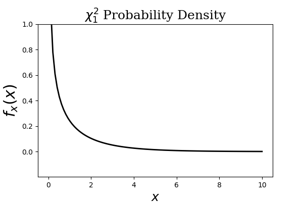
The $\chi_1^2$ density has much # of its weight on the left, which is excluded in the establishment of the Markov # Inequality.
# #
#
#
#
#
#
#
#
#
#
#
#
#
#
#
#
#
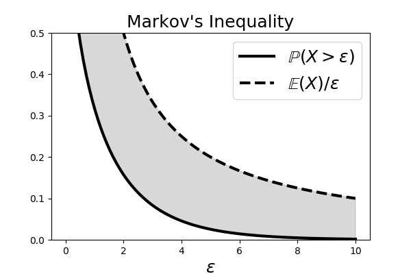
# The shaded area # shows the region between the curves on either side of the Markov Inequality.
# #
#
#
#
# ## Chebyshev's Inequality
#
# Chebyshev's Inequality drops out
# directly from the Markov Inequality. Let
# $\mu=\mathbb{E}(X)$ and
# $\sigma^2=\mathbb{V}(X)$. Then, we have
#
# $$
# \mathbb{P}(\vert X-\mu\vert \ge t) \le \frac{\sigma^2}{t^2}
# $$
#
# Note that if we normalize so that $Z=(X-\mu)/\sigma$, we
# have $\mathbb{P}(\vert
# Z\vert \ge k) \le 1/k^2$. In particular,
# $\mathbb{P}(\vert Z\vert \ge 2) \le
# 1/4$. We can illustrate this
# inequality using Sympy statistics module,
# In[2]:
import sympy
import sympy.stats as ss
t=sympy.symbols('t',real=True)
x=ss.ChiSquared('x',1)
# To get the left side of the Chebyshev inequality, we
# have to write this out as
# the following conditional probability,
# In[3]:
r = ss.P((x-1) > t,x>1)+ss.P(-(x-1) > t,x<1)
# We could take the above expression, which is a function of $t$ and
# attempt to
# compute the integral, but that would take a very long time (the
# expression is
# very long and complicated, which is why we did not print it out
# above). In this
# situation, it's better to use the built-in cumulative density
# function as in the
# following (after some rearrangement of the terms),
# In[4]:
w=(1-ss.cdf(x)(t+1))+ss.cdf(x)(1-t)
# To plot this, we can evaluated at a variety of `t` values by using
# the `.subs`
# substitution method, but it is more convenient to use the
# `lambdify` method to
# convert the expression to a function.
# In[5]:
fw=sympy.lambdify(t,w)
# Then, we can evaluate this function using something like
# In[6]:
[fw(i) for i in [0,1,2,3,4,5]]
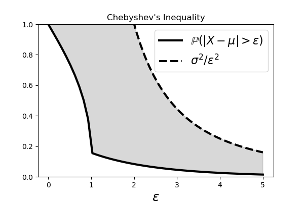
# to produce the following [Figure](#fig:ProbabilityInequalities_003).
#
#
#
#
#
#
#
#
#
#
# ## Chebyshev's Inequality
#
# Chebyshev's Inequality drops out
# directly from the Markov Inequality. Let
# $\mu=\mathbb{E}(X)$ and
# $\sigma^2=\mathbb{V}(X)$. Then, we have
#
# $$
# \mathbb{P}(\vert X-\mu\vert \ge t) \le \frac{\sigma^2}{t^2}
# $$
#
# Note that if we normalize so that $Z=(X-\mu)/\sigma$, we
# have $\mathbb{P}(\vert
# Z\vert \ge k) \le 1/k^2$. In particular,
# $\mathbb{P}(\vert Z\vert \ge 2) \le
# 1/4$. We can illustrate this
# inequality using Sympy statistics module,
# In[2]:
import sympy
import sympy.stats as ss
t=sympy.symbols('t',real=True)
x=ss.ChiSquared('x',1)
# To get the left side of the Chebyshev inequality, we
# have to write this out as
# the following conditional probability,
# In[3]:
r = ss.P((x-1) > t,x>1)+ss.P(-(x-1) > t,x<1)
# We could take the above expression, which is a function of $t$ and
# attempt to
# compute the integral, but that would take a very long time (the
# expression is
# very long and complicated, which is why we did not print it out
# above). In this
# situation, it's better to use the built-in cumulative density
# function as in the
# following (after some rearrangement of the terms),
# In[4]:
w=(1-ss.cdf(x)(t+1))+ss.cdf(x)(1-t)
# To plot this, we can evaluated at a variety of `t` values by using
# the `.subs`
# substitution method, but it is more convenient to use the
# `lambdify` method to
# convert the expression to a function.
# In[5]:
fw=sympy.lambdify(t,w)
# Then, we can evaluate this function using something like
# In[6]:
[fw(i) for i in [0,1,2,3,4,5]]
# to produce the following [Figure](#fig:ProbabilityInequalities_003).
#
#
#
#
#
# The # shaded area shows the region between the curves on either side of the Chebyshev # Inequality.
# #
#
#
#
# **Programming Tip.**
#
# Note that we cannot use
# vectorized inputs for the `lambdify` function because
# it contains embedded
# functions that are only available in Sympy. Otherwise, we
# could have used
# `lambdify(t,fw,numpy)` to specify the corresponding functions
# in Numpy to use
# for the expression.
#
#
#
# ## Hoeffding's Inequality
#
#
# Hoeffding's Inequality is similar, but less loose,
# than Markov's Inequality.
# Let $X_1,\ldots,X_n$ be iid observations such that
# $\mathbb{E}(X_i)=\mu$ and
# $a\le X_i \le b$. Then, for any $\epsilon>0$, we have
#
# $$
# \mathbb{P}(\vert \overline{X}_n -\mu\vert \ge \epsilon) \le 2 \exp(-2
# n\epsilon^2/(b-a)^2)
# $$
#
# where $\overline{X}_n = \tfrac{1}{n}\sum_i^n X_i$. Note that we
# further assume
# that the individual random variables are bounded.
#
# **Corollary.** If
# $X_1,\ldots,X_n$ are independent with $\mathbb{P}(a\le X_i\le b)=1$
# and all with
# $\mathbb{E}(X_i)=\mu$. Then, we have
#
# $$
# \vert\overline{X}_n-\mu\vert \le \sqrt{\frac{c}{2 n}\log \frac{2}{\delta}}
# $$
#
# where $c=(b-a)^2$. We will see this inequality again in the machine
# learning
# chapter. [Figure](#fig:ProbabilityInequalities_004) shows the Markov
# and
# Hoeffding bounds for the case of ten identically and uniformly distributed
# random variables, $X_i \sim \mathcal{U}[0,1]$. The solid line shows
# $\mathbb{P}(\vert \overline{X}_n - 1/2 \vert > \epsilon)$. Note that the
# Hoeffding Inequality is tighter than the Markov Inequality and that both of
# them
# merge when $\epsilon$ gets big enough.
#
#
#
#
#
#
#
#
#
# **Programming Tip.**
#
# Note that we cannot use
# vectorized inputs for the `lambdify` function because
# it contains embedded
# functions that are only available in Sympy. Otherwise, we
# could have used
# `lambdify(t,fw,numpy)` to specify the corresponding functions
# in Numpy to use
# for the expression.
#
#
#
# ## Hoeffding's Inequality
#
#
# Hoeffding's Inequality is similar, but less loose,
# than Markov's Inequality.
# Let $X_1,\ldots,X_n$ be iid observations such that
# $\mathbb{E}(X_i)=\mu$ and
# $a\le X_i \le b$. Then, for any $\epsilon>0$, we have
#
# $$
# \mathbb{P}(\vert \overline{X}_n -\mu\vert \ge \epsilon) \le 2 \exp(-2
# n\epsilon^2/(b-a)^2)
# $$
#
# where $\overline{X}_n = \tfrac{1}{n}\sum_i^n X_i$. Note that we
# further assume
# that the individual random variables are bounded.
#
# **Corollary.** If
# $X_1,\ldots,X_n$ are independent with $\mathbb{P}(a\le X_i\le b)=1$
# and all with
# $\mathbb{E}(X_i)=\mu$. Then, we have
#
# $$
# \vert\overline{X}_n-\mu\vert \le \sqrt{\frac{c}{2 n}\log \frac{2}{\delta}}
# $$
#
# where $c=(b-a)^2$. We will see this inequality again in the machine
# learning
# chapter. [Figure](#fig:ProbabilityInequalities_004) shows the Markov
# and
# Hoeffding bounds for the case of ten identically and uniformly distributed
# random variables, $X_i \sim \mathcal{U}[0,1]$. The solid line shows
# $\mathbb{P}(\vert \overline{X}_n - 1/2 \vert > \epsilon)$. Note that the
# Hoeffding Inequality is tighter than the Markov Inequality and that both of
# them
# merge when $\epsilon$ gets big enough.
#
#
#
#
# This shows the Markov and Hoeffding bounds for the case of ten identically # and uniformly distributed random variables.
# #
#
# ### Proof of Hoeffding's Inequality
#
# We will need the following lemma to prove
# Hoeffding's inequality.
#
# **Lemma** Let $X$ be a random variable with
# $\mathbb{E}(X)=0$ and
# $a\le X\le b$. Then, for any $s>0$, we have the following,
#
#
#
#
# $$
# \begin{equation}
# \mathbb{E}(e^{s X}) \le e^{s^2(b-a)^2/8}
# \label{_auto1} \tag{1}
# \end{equation}
# $$
#
# Because $X$ is contained in the closed interval $[a,b]$, we can write it as a
# convex
# combination of the endpoints of the interval.
#
# $$
# X = \alpha_1 a + \alpha_2 b
# $$
#
# where $\alpha_1+\alpha_2=1$. Solving for the $\alpha_i$ terms, we have
#
# $$
# \begin{align*}
# \alpha_1 = & \frac{x-a}{b-a} \\
# \alpha_2 = &
# \frac{b-x}{b-a}
# \end{align*}
# $$
#
# From Jensen's inequality, for a convex functions $f$, we know that
#
# $$
# f\left(\sum \alpha_i x_i\right) \le \sum \alpha_i f(x_i)
# $$
#
# Given the convexity of $e^X$, we therefore have,
#
# $$
# e^{s X} \le \alpha_1 e^{s a} + \alpha_2 e^ {s b}
# $$
#
# With $\mathbb{E}(X)=0$, we can write the expectation of both sides
#
# $$
# \mathbb{E}(e^{s X}) \le \mathbb{E}(\alpha_1) e^{s a}
# +\mathbb{E}(\alpha_2) e^{s b}
# $$
#
# with $\mathbb{E}(\alpha_1)=\frac{b}{b-a}$ and
# $\mathbb{E}(\alpha_2)=\frac{-a}{b-a}$. Thus, we have
#
# $$
# \mathbb{E}(e^{s X}) \le \frac{b}{b-a} e^{s a} -\frac{a}{b-a} e^{s b}
# $$
#
# Using $p:=\frac{-a}{b-a}$, we can rewrite the following,
#
# $$
# \frac{b}{b-a} e^{s a} -\frac{a}{b-a} e^{s b} = (1-p)e^{s a} + p e^{s b} =:
# e^{\phi(u)}
# $$
#
# where
#
# $$
# \phi(u)=-p u + \log(1-p+p e^{u})
# $$
#
# and $u=s(b-a)$. Note that $\phi(0)=\phi'(0)=0$. Also, $\phi''(0) = p(1-p)\le
# 1/4$. Thus,
# the Taylor expansion of $\phi(u)\approx \frac{u^2}{2}\phi''(t) \le
# \frac{u^2}{8}$ for
# $t\in [0,u] \blacksquare$.
#
# To prove Hoeffding's inequality,
# we start with Markov's inequality,
#
# $$
# \mathbb{P}(X\ge\epsilon)\le \frac{\mathbb{E}(X)}{\epsilon}
# $$
#
# Then, given $s>0$, we have the following,
#
# $$
# \mathbb{P}(X\ge\epsilon)=\mathbb{P}(e^{s X} \ge e^{s\epsilon}) \le
# \frac{\mathbb{E}(e^{s X})}{e^{s \epsilon}}
# $$
#
# We can write the one-sided Hoeffding inequality as the following,
#
# $$
# \begin{align*}
# \mathbb{P}(\overline{X}_n -\mu\ge\epsilon) & \le
# e^{-s\epsilon}\mathbb{E}(\exp(\frac{s}{n}\sum_{i=1}^n (X_i-\mathbb{E}(X_i)))) \\
# & = e^{-s\epsilon}\prod_{i=1}^n\mathbb{E}(e^{ \frac{s}{n} (X_i-\mathbb{E}(X_i))
# }) \\
# & \le e^{-s\epsilon}\prod_{i=1}^n e^{\frac{s^2}{n^2}(b-a)^2/8 } \\
# & = e^{-s\epsilon} e^{\frac{s^2}{n}(b-a)^2/8}
# \end{align*}
# $$
#
# Now, we want to pick $s>0$ to minimize this upper bound. Then, with
# $s=\frac{4
# n\epsilon}{(b-a)^2}$
#
# $$
# \mathbb{P}(\overline{X}_n-\mu\ge\epsilon)\le e^{-\frac{2
# n\epsilon^2}{(b-a)^2}}
# $$
#
# The other side of the inequality follows similarly to obtain Hoeffding's
# inequality $\blacksquare$.
#
# ## Jensen's Inequality
#
#
# If $f$ is a convex function with random variable
# $v$, then
#
# $$
# \mathbb{E}(f(v))\ge f(\mathbb{E}(v))
# $$
#
# The proof of this is straightforward. Define $L(v) = a v +b $ with
# $a,b\in
# \mathbb{R}$. Choose $a$ and $b$ so that
# $L(\mathbb{E}(v))=f(\mathbb{E}(v))$
# which makes $L$ tangent to $f$ at
# $\mathbb{E}(v)$. By the convexity of $f$, we
# have $f(v)\ge L(v)$. We can take
# the expectation of both sides of this,
#
# $$
# \begin{align*}
# \mathbb{E}(f(v)) \ge & \mathbb{E}(L(v)) \\
# =
# & \mathbb{E}(a v+b) \\
# = & a\mathbb{E}(v)+b \\
# = & L(\mathbb{E}(v)) \\
# = & f(\mathbb{E}(v))
# \end{align*}
# $$
#
# equality holds when $f$ is linear. For a concave function $f$, the
# sense of the
# inequality is reversed.
#
# In[ ]:
#
#
# ### Proof of Hoeffding's Inequality
#
# We will need the following lemma to prove
# Hoeffding's inequality.
#
# **Lemma** Let $X$ be a random variable with
# $\mathbb{E}(X)=0$ and
# $a\le X\le b$. Then, for any $s>0$, we have the following,
#
#
#
#
# $$
# \begin{equation}
# \mathbb{E}(e^{s X}) \le e^{s^2(b-a)^2/8}
# \label{_auto1} \tag{1}
# \end{equation}
# $$
#
# Because $X$ is contained in the closed interval $[a,b]$, we can write it as a
# convex
# combination of the endpoints of the interval.
#
# $$
# X = \alpha_1 a + \alpha_2 b
# $$
#
# where $\alpha_1+\alpha_2=1$. Solving for the $\alpha_i$ terms, we have
#
# $$
# \begin{align*}
# \alpha_1 = & \frac{x-a}{b-a} \\
# \alpha_2 = &
# \frac{b-x}{b-a}
# \end{align*}
# $$
#
# From Jensen's inequality, for a convex functions $f$, we know that
#
# $$
# f\left(\sum \alpha_i x_i\right) \le \sum \alpha_i f(x_i)
# $$
#
# Given the convexity of $e^X$, we therefore have,
#
# $$
# e^{s X} \le \alpha_1 e^{s a} + \alpha_2 e^ {s b}
# $$
#
# With $\mathbb{E}(X)=0$, we can write the expectation of both sides
#
# $$
# \mathbb{E}(e^{s X}) \le \mathbb{E}(\alpha_1) e^{s a}
# +\mathbb{E}(\alpha_2) e^{s b}
# $$
#
# with $\mathbb{E}(\alpha_1)=\frac{b}{b-a}$ and
# $\mathbb{E}(\alpha_2)=\frac{-a}{b-a}$. Thus, we have
#
# $$
# \mathbb{E}(e^{s X}) \le \frac{b}{b-a} e^{s a} -\frac{a}{b-a} e^{s b}
# $$
#
# Using $p:=\frac{-a}{b-a}$, we can rewrite the following,
#
# $$
# \frac{b}{b-a} e^{s a} -\frac{a}{b-a} e^{s b} = (1-p)e^{s a} + p e^{s b} =:
# e^{\phi(u)}
# $$
#
# where
#
# $$
# \phi(u)=-p u + \log(1-p+p e^{u})
# $$
#
# and $u=s(b-a)$. Note that $\phi(0)=\phi'(0)=0$. Also, $\phi''(0) = p(1-p)\le
# 1/4$. Thus,
# the Taylor expansion of $\phi(u)\approx \frac{u^2}{2}\phi''(t) \le
# \frac{u^2}{8}$ for
# $t\in [0,u] \blacksquare$.
#
# To prove Hoeffding's inequality,
# we start with Markov's inequality,
#
# $$
# \mathbb{P}(X\ge\epsilon)\le \frac{\mathbb{E}(X)}{\epsilon}
# $$
#
# Then, given $s>0$, we have the following,
#
# $$
# \mathbb{P}(X\ge\epsilon)=\mathbb{P}(e^{s X} \ge e^{s\epsilon}) \le
# \frac{\mathbb{E}(e^{s X})}{e^{s \epsilon}}
# $$
#
# We can write the one-sided Hoeffding inequality as the following,
#
# $$
# \begin{align*}
# \mathbb{P}(\overline{X}_n -\mu\ge\epsilon) & \le
# e^{-s\epsilon}\mathbb{E}(\exp(\frac{s}{n}\sum_{i=1}^n (X_i-\mathbb{E}(X_i)))) \\
# & = e^{-s\epsilon}\prod_{i=1}^n\mathbb{E}(e^{ \frac{s}{n} (X_i-\mathbb{E}(X_i))
# }) \\
# & \le e^{-s\epsilon}\prod_{i=1}^n e^{\frac{s^2}{n^2}(b-a)^2/8 } \\
# & = e^{-s\epsilon} e^{\frac{s^2}{n}(b-a)^2/8}
# \end{align*}
# $$
#
# Now, we want to pick $s>0$ to minimize this upper bound. Then, with
# $s=\frac{4
# n\epsilon}{(b-a)^2}$
#
# $$
# \mathbb{P}(\overline{X}_n-\mu\ge\epsilon)\le e^{-\frac{2
# n\epsilon^2}{(b-a)^2}}
# $$
#
# The other side of the inequality follows similarly to obtain Hoeffding's
# inequality $\blacksquare$.
#
# ## Jensen's Inequality
#
#
# If $f$ is a convex function with random variable
# $v$, then
#
# $$
# \mathbb{E}(f(v))\ge f(\mathbb{E}(v))
# $$
#
# The proof of this is straightforward. Define $L(v) = a v +b $ with
# $a,b\in
# \mathbb{R}$. Choose $a$ and $b$ so that
# $L(\mathbb{E}(v))=f(\mathbb{E}(v))$
# which makes $L$ tangent to $f$ at
# $\mathbb{E}(v)$. By the convexity of $f$, we
# have $f(v)\ge L(v)$. We can take
# the expectation of both sides of this,
#
# $$
# \begin{align*}
# \mathbb{E}(f(v)) \ge & \mathbb{E}(L(v)) \\
# =
# & \mathbb{E}(a v+b) \\
# = & a\mathbb{E}(v)+b \\
# = & L(\mathbb{E}(v)) \\
# = & f(\mathbb{E}(v))
# \end{align*}
# $$
#
# equality holds when $f$ is linear. For a concave function $f$, the
# sense of the
# inequality is reversed.
#
# In[ ]: