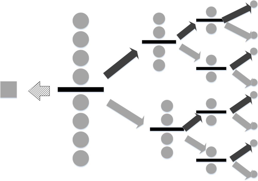
One heavy # ball is hidden among eight identical balls. By weighing groups sequentially, we # can determine the heavy ball.
# #
#
#
#
# If we get lucky, the scale will report that
# the group of four walls on either
# side of the balance are equal in weight. This
# means that the ball that was
# omitted is the heavier one. This is indicated by
# the hashed left-pointing
# arrow. In this case, all the uncertainty has
# evaporated, and the *informational
# value* of that one weighing is equal to
# $\log_2(9)$. In other words, the scale
# has reduced the uncertainty to zero
# (i.e., found the heavy ball). On the other
# hand, the scale could report that the
# upper group of four balls is heavier
# (black, upward-pointing arrow) or lighter
# (gray, downward-pointing arrow). In
# this case, we cannot isolate the heavier
# ball until we perform all of the
# indicated weighings, moving from left-to-right.
# Specifically, the four balls on
# the heavier side have to be split by a
# subsequent weighing into two balls and
# then to one ball before the heavy ball
# can be identified. Thus, this process
# takes three weighings. The first one has
# information content $\log_2(9/8)$, the
# next has $\log_2(4)$, and the final one
# has $\log_2(2)$. Adding all these up
# sums to $\log_2(9)$. Thus, whether or not
# the heavier ball is isolated in the
# first weighing, the strategy consumes
# $\log_2(9)$ bits, as it must, to find the
# heavy ball.
#
#
#
#
#
#
#
#
#
#
# If we get lucky, the scale will report that
# the group of four walls on either
# side of the balance are equal in weight. This
# means that the ball that was
# omitted is the heavier one. This is indicated by
# the hashed left-pointing
# arrow. In this case, all the uncertainty has
# evaporated, and the *informational
# value* of that one weighing is equal to
# $\log_2(9)$. In other words, the scale
# has reduced the uncertainty to zero
# (i.e., found the heavy ball). On the other
# hand, the scale could report that the
# upper group of four balls is heavier
# (black, upward-pointing arrow) or lighter
# (gray, downward-pointing arrow). In
# this case, we cannot isolate the heavier
# ball until we perform all of the
# indicated weighings, moving from left-to-right.
# Specifically, the four balls on
# the heavier side have to be split by a
# subsequent weighing into two balls and
# then to one ball before the heavy ball
# can be identified. Thus, this process
# takes three weighings. The first one has
# information content $\log_2(9/8)$, the
# next has $\log_2(4)$, and the final one
# has $\log_2(2)$. Adding all these up
# sums to $\log_2(9)$. Thus, whether or not
# the heavier ball is isolated in the
# first weighing, the strategy consumes
# $\log_2(9)$ bits, as it must, to find the
# heavy ball.
#
#
#
#
#
# For this strategy, the balls are # broken up into three groups of equal size and subsequently weighed.
# #
#
#
#
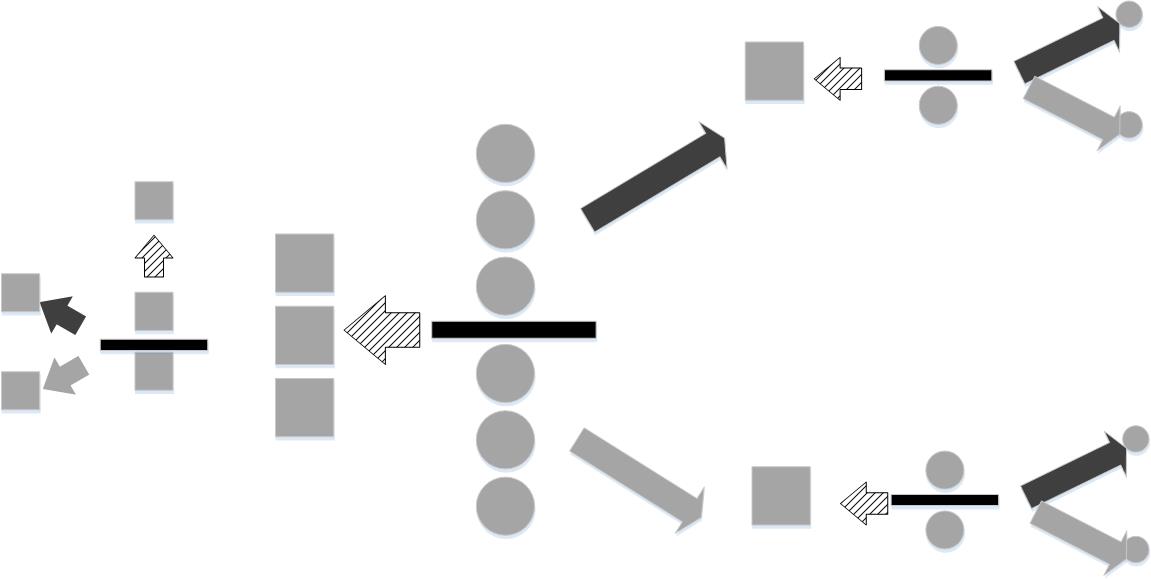
# However,
# this is not the only strategy. [Figure](#fig:Information_Entropy_002)
# shows
# another. In this approach, the nine balls are split up into three groups
# of
# three balls apiece. Two groups are weighed. If they are of equal weight,
# then
# this means the heavier ball is in the group that was left out (dashed
# arrow).
# Then, this group is split into two groups, with one element left out.
# If the two
# balls on the scale weigh the same, then it means the excluded one is
# the heavy
# one. Otherwise, it is one of the balls on the scale. The same process
# follows if
# one of the initially weighed groups is heavier (black upward-facing
# arrow) or
# lighter (gray lower-facing arrow). As before the information content
# of the
# situation is $\log_2(9)$. The first weighing reduces the uncertainty of
# the
# situation by $\log_2(3)$ and the subsequent weighing reduces it by another
# $\log_2(3)$. As before, these sum to $\log_2(9)$, but here we only need two
# weighings whereas the first strategy in [Figure](#fig:Information_Entropy_001)
# takes
# an average of $1/9 + 3*8/9 \approx 2.78$ weighings, which is more than two
# from the second strategy in [Figure](#fig:Information_Entropy_002).
#
# Why does
# the second strategy use fewer weighings? To reduce weighings, we need
# each
# weighing to adjudicate equally probable situations as many times as
# possible.
# Choosing one of the nine balls at the outset (i.e, first strategy in
# [Figure](#fig:Information_Entropy_001)) does not do this because the
# probability
# of selecting the correct ball is $1/9$. This does not create a
# equiprobable
# situation in the process. The second strategy leaves an equally
# probable
# situation at every stage (see [Figure](#fig:Information_Entropy_002)), so it
# extracts the most information out of
# each weighing as possible. Thus, the
# information content tells us how many bits
# of information have to be resolved
# using *any* strategy (i.e., $\log_2(9)$ in
# this example). It also illuminates
# how to efficiently remove uncertainty;
# namely, by adjudicating equiprobable
# situations as many times as possible.
#
# ## Properties of Information Entropy
# Now that we have the flavor of the concepts, consider the following properties
# of the information entropy,
#
# $$
# H(X) \ge 0
# $$
#
# with equality if and only if $P(x)=1$ for exactly one $x$.
# Intuitively, this
# means that when just one of the items in the ensemble is
# known absolutely (i.e.,
# with $P(x)=1$), the uncertainty collapses to zero.
# Also note that entropy is
# maximized when $P$ is uniformly distributed across
# the elements of the ensemble.
# This is illustrated in [Figure](#fig:Information_Entropy_003) for the case of
# two outcomes. In other words,
# information entropy is maximized when the two
# conflicting alternatives are
# equally probable. This is the mathematical reason
# why using the scale in the
# last example to adjudicate equally probable
# situations was so useful for
# abbreviating the weighing process.
# In[4]:
get_ipython().run_line_magic('matplotlib', 'inline')
from matplotlib.pylab import subplots
import numpy as np
p = np.linspace(0.001,1-.001,50)
fig,ax=subplots()
#fig.set_size_inches((14,7))
_=ax.plot(p,p*np.log2(1/p)+(1-p)*np.log2(1/(1-p)),'k-')
_=ax.set_xlabel('$p$',fontsize=24)
_=ax.set_ylabel('$H(p)$',fontsize=24)
_=ax.grid()
fig.tight_layout()
fig.savefig('fig-probability/information_entropy_003.png')
#
#
#
#
#
#
#
#
#
# However,
# this is not the only strategy. [Figure](#fig:Information_Entropy_002)
# shows
# another. In this approach, the nine balls are split up into three groups
# of
# three balls apiece. Two groups are weighed. If they are of equal weight,
# then
# this means the heavier ball is in the group that was left out (dashed
# arrow).
# Then, this group is split into two groups, with one element left out.
# If the two
# balls on the scale weigh the same, then it means the excluded one is
# the heavy
# one. Otherwise, it is one of the balls on the scale. The same process
# follows if
# one of the initially weighed groups is heavier (black upward-facing
# arrow) or
# lighter (gray lower-facing arrow). As before the information content
# of the
# situation is $\log_2(9)$. The first weighing reduces the uncertainty of
# the
# situation by $\log_2(3)$ and the subsequent weighing reduces it by another
# $\log_2(3)$. As before, these sum to $\log_2(9)$, but here we only need two
# weighings whereas the first strategy in [Figure](#fig:Information_Entropy_001)
# takes
# an average of $1/9 + 3*8/9 \approx 2.78$ weighings, which is more than two
# from the second strategy in [Figure](#fig:Information_Entropy_002).
#
# Why does
# the second strategy use fewer weighings? To reduce weighings, we need
# each
# weighing to adjudicate equally probable situations as many times as
# possible.
# Choosing one of the nine balls at the outset (i.e, first strategy in
# [Figure](#fig:Information_Entropy_001)) does not do this because the
# probability
# of selecting the correct ball is $1/9$. This does not create a
# equiprobable
# situation in the process. The second strategy leaves an equally
# probable
# situation at every stage (see [Figure](#fig:Information_Entropy_002)), so it
# extracts the most information out of
# each weighing as possible. Thus, the
# information content tells us how many bits
# of information have to be resolved
# using *any* strategy (i.e., $\log_2(9)$ in
# this example). It also illuminates
# how to efficiently remove uncertainty;
# namely, by adjudicating equiprobable
# situations as many times as possible.
#
# ## Properties of Information Entropy
# Now that we have the flavor of the concepts, consider the following properties
# of the information entropy,
#
# $$
# H(X) \ge 0
# $$
#
# with equality if and only if $P(x)=1$ for exactly one $x$.
# Intuitively, this
# means that when just one of the items in the ensemble is
# known absolutely (i.e.,
# with $P(x)=1$), the uncertainty collapses to zero.
# Also note that entropy is
# maximized when $P$ is uniformly distributed across
# the elements of the ensemble.
# This is illustrated in [Figure](#fig:Information_Entropy_003) for the case of
# two outcomes. In other words,
# information entropy is maximized when the two
# conflicting alternatives are
# equally probable. This is the mathematical reason
# why using the scale in the
# last example to adjudicate equally probable
# situations was so useful for
# abbreviating the weighing process.
# In[4]:
get_ipython().run_line_magic('matplotlib', 'inline')
from matplotlib.pylab import subplots
import numpy as np
p = np.linspace(0.001,1-.001,50)
fig,ax=subplots()
#fig.set_size_inches((14,7))
_=ax.plot(p,p*np.log2(1/p)+(1-p)*np.log2(1/(1-p)),'k-')
_=ax.set_xlabel('$p$',fontsize=24)
_=ax.set_ylabel('$H(p)$',fontsize=24)
_=ax.grid()
fig.tight_layout()
fig.savefig('fig-probability/information_entropy_003.png')
#
#
#
#
# The information entropy is maximized # when $p=1/2$.
# #
#
#
#
# Most importantly, the concept of entropy
# extends jointly as follows,
#
# $$
# H(X,Y) = \sum_{x,y} P(x,y) \log_2 \frac{1}{P(x,y)}
# $$
#
# If and only if $X$ and $Y$ are independent, entropy becomes
# additive,
#
# $$
# H(X,Y) = H(X)+H(Y)
# $$
#
# ## Kullback-Leibler Divergence
#
# Notions of information entropy lead to notions
# of distance between probability
# distributions that will become important for
# machine learning methods. The
# Kullback-Leibler divergence between two
# probability distributions $P$ and $Q$
# that are defined over the same set is
# defined as,
#
# $$
# D_{KL}(P,Q) = \sum_x P(x) \log_2 \frac{P(x)}{Q(x)}
# $$
#
# Note that $D_{KL}(P,Q) \ge 0$ with equality if and only if $P=Q$.
# Sometimes the
# Kullback-Leibler divergence is called the Kullback-Leibler
# distance, but it is
# not formally a distance metric because it is asymmetrical
# in $P$ and $Q$. The
# Kullback-Leibler divergence defines a relative entropy as
# the loss of
# information if $P$ is modeled in terms of $Q$. There is an
# intuitive way to
# interpret the Kullback-Leibler divergence and understand its
# lack of symmetry.
# Suppose we have a set of messages to transmit, each with a
# corresponding
# probability $\lbrace
# (x_1,P(x_1)),(x_2,P(x_2)),\ldots,(x_n,P(x_n)) \rbrace$.
# Based on what we know
# about information entropy, it makes sense to encode the
# length of the message
# by $\log_2 \frac{1}{p(x)}$ bits. This parsimonious
# strategy means that more
# frequent messages are encoded with fewer bits. Thus, we
# can rewrite the entropy
# of the situation as before,
#
# $$
# H(X) = \sum_{k} P(x_k) \log_2 \frac{1}{P(x_k)}
# $$
#
# Now, suppose we want to transmit the same set of messages, but with a
# different
# set of probability weights, $\lbrace
# (x_1,Q(x_1)),(x_2,Q(x_2)),\ldots,(x_n,Q(x_n)) \rbrace$. In this situation, we
# can define the cross-entropy as
#
# $$
# H_q(X) = \sum_{k} P(x_k) \log_2 \frac{1}{Q(x_k)}
# $$
#
# Note that only the purported length of the encoded message has
# changed, not the
# probability of that message. The difference between these two
# is the Kullback-
# Leibler divergence,
#
# $$
# D_{KL}(P,Q)=H_q(X)-H(X)=\sum_x P(x) \log_2 \frac{P(x)}{Q(x)}
# $$
#
# In this light, the Kullback-Leibler divergence is the average
# difference in the
# encoded lengths of the same set of messages under two
# different probability
# regimes. This should help explain the lack of symmetry of
# the Kullback-Leibler
# divergence --- left to themselves, $P$ and $Q$ would
# provide the optimal-length
# encodings separately, but there can be no necessary
# symmetry in how each regime
# would rate the informational value of each message
# ($Q(x_i)$ versus $P(x_i)$).
# Given that each encoding is optimal-length in its
# own regime means that it must
# therefore be at least sub-optimal in another,
# thus giving rise to the Kullback-
# Leibler divergence. In the case where the
# encoding length of all messages
# remains the same for the two regimes, then the
# Kullback-Leibler divergence is
# zero [^Mackay].
#
# [^Mackay]: The best, easy-to-understand presentation of this
# material is chapter
# four of Mackay's text
# [[mackay2003information]](#mackay2003information). Another good reference is
# chapter four of [[hastie2013elements]](#hastie2013elements).
#
#
# ## Cross-Entropy
# as Maximum Likelihood
#
#
#
# Reconsidering maximum
# likelihood from our statistics chapter in more
# general terms, we have
#
# $$
# \theta_{\texttt{ML}} =\argmax_{\theta} \sum_{i=1}^n \log
# p_{\texttt{model}}(x_i;\theta)
# $$
#
# where $p_{\texttt{model}}$ is the assumed underlying probability
# density
# function parameterized by $\theta$ for the $x_i$ data elements.
# Dividing the
# above summation by $n$ does not change the derived optimal values,
# but it allows
# us to rewrite this using the empirical density function for $x$
# as the
# following,
#
# $$
# \theta_{\texttt{ML}} = \argmax_{\theta} \mathbb{E}_{x\sim
# \hat{p}_{\texttt{data}}}(\log p_{\texttt{model}}(x_i;\theta))
# $$
#
# Note that we have the distinction between $p_{\texttt{data}}$ and
# $\hat{p}_{\texttt{data}}$ where the former is the unknown distribution of
# the data and the latter is the estimated distribution of the data we have on
# hand.
#
# The cross-entropy can be written as the following,
#
# $$
# D_{KL}(P,Q) = \mathbb{E}_{X\sim P}(\log P(x))-\mathbb{E}_{X\sim P}(\log Q(x))
# $$
#
# where $X\sim P$ means the random variable $X$ has distribution $P$.
# Thus, we
# have
#
# $$
# \theta_{\texttt{ML}} = \argmax_{\theta}
# D_{KL}(\hat{p}_{\texttt{data}}, p_{\texttt{model}})
# $$
#
# That is, we can interpret maximum likelihood as the cross-entropy
# between the
# $p_{\texttt{model}}$ and the $\hat{p}_{\texttt{data}}$
# distributions.
# The first term has nothing to do with the estimated $\theta$ so
# maximizing this
# is the same as minimizing the following,
#
# $$
# \mathbb{E}_{x\sim \hat{p}_{\texttt{data}}}(\log
# p_{\texttt{model}}(x_i;\theta))
# $$
#
# because information entropy is always non-negative. The important
# interpretation is that maximum likelihood is an attempt to choose $\theta$
# model
# parameters that make the empirical distribution of the data match the
# model
# distribution.
#
#
#
#
# Most importantly, the concept of entropy
# extends jointly as follows,
#
# $$
# H(X,Y) = \sum_{x,y} P(x,y) \log_2 \frac{1}{P(x,y)}
# $$
#
# If and only if $X$ and $Y$ are independent, entropy becomes
# additive,
#
# $$
# H(X,Y) = H(X)+H(Y)
# $$
#
# ## Kullback-Leibler Divergence
#
# Notions of information entropy lead to notions
# of distance between probability
# distributions that will become important for
# machine learning methods. The
# Kullback-Leibler divergence between two
# probability distributions $P$ and $Q$
# that are defined over the same set is
# defined as,
#
# $$
# D_{KL}(P,Q) = \sum_x P(x) \log_2 \frac{P(x)}{Q(x)}
# $$
#
# Note that $D_{KL}(P,Q) \ge 0$ with equality if and only if $P=Q$.
# Sometimes the
# Kullback-Leibler divergence is called the Kullback-Leibler
# distance, but it is
# not formally a distance metric because it is asymmetrical
# in $P$ and $Q$. The
# Kullback-Leibler divergence defines a relative entropy as
# the loss of
# information if $P$ is modeled in terms of $Q$. There is an
# intuitive way to
# interpret the Kullback-Leibler divergence and understand its
# lack of symmetry.
# Suppose we have a set of messages to transmit, each with a
# corresponding
# probability $\lbrace
# (x_1,P(x_1)),(x_2,P(x_2)),\ldots,(x_n,P(x_n)) \rbrace$.
# Based on what we know
# about information entropy, it makes sense to encode the
# length of the message
# by $\log_2 \frac{1}{p(x)}$ bits. This parsimonious
# strategy means that more
# frequent messages are encoded with fewer bits. Thus, we
# can rewrite the entropy
# of the situation as before,
#
# $$
# H(X) = \sum_{k} P(x_k) \log_2 \frac{1}{P(x_k)}
# $$
#
# Now, suppose we want to transmit the same set of messages, but with a
# different
# set of probability weights, $\lbrace
# (x_1,Q(x_1)),(x_2,Q(x_2)),\ldots,(x_n,Q(x_n)) \rbrace$. In this situation, we
# can define the cross-entropy as
#
# $$
# H_q(X) = \sum_{k} P(x_k) \log_2 \frac{1}{Q(x_k)}
# $$
#
# Note that only the purported length of the encoded message has
# changed, not the
# probability of that message. The difference between these two
# is the Kullback-
# Leibler divergence,
#
# $$
# D_{KL}(P,Q)=H_q(X)-H(X)=\sum_x P(x) \log_2 \frac{P(x)}{Q(x)}
# $$
#
# In this light, the Kullback-Leibler divergence is the average
# difference in the
# encoded lengths of the same set of messages under two
# different probability
# regimes. This should help explain the lack of symmetry of
# the Kullback-Leibler
# divergence --- left to themselves, $P$ and $Q$ would
# provide the optimal-length
# encodings separately, but there can be no necessary
# symmetry in how each regime
# would rate the informational value of each message
# ($Q(x_i)$ versus $P(x_i)$).
# Given that each encoding is optimal-length in its
# own regime means that it must
# therefore be at least sub-optimal in another,
# thus giving rise to the Kullback-
# Leibler divergence. In the case where the
# encoding length of all messages
# remains the same for the two regimes, then the
# Kullback-Leibler divergence is
# zero [^Mackay].
#
# [^Mackay]: The best, easy-to-understand presentation of this
# material is chapter
# four of Mackay's text
# [[mackay2003information]](#mackay2003information). Another good reference is
# chapter four of [[hastie2013elements]](#hastie2013elements).
#
#
# ## Cross-Entropy
# as Maximum Likelihood
#
#
#
# Reconsidering maximum
# likelihood from our statistics chapter in more
# general terms, we have
#
# $$
# \theta_{\texttt{ML}} =\argmax_{\theta} \sum_{i=1}^n \log
# p_{\texttt{model}}(x_i;\theta)
# $$
#
# where $p_{\texttt{model}}$ is the assumed underlying probability
# density
# function parameterized by $\theta$ for the $x_i$ data elements.
# Dividing the
# above summation by $n$ does not change the derived optimal values,
# but it allows
# us to rewrite this using the empirical density function for $x$
# as the
# following,
#
# $$
# \theta_{\texttt{ML}} = \argmax_{\theta} \mathbb{E}_{x\sim
# \hat{p}_{\texttt{data}}}(\log p_{\texttt{model}}(x_i;\theta))
# $$
#
# Note that we have the distinction between $p_{\texttt{data}}$ and
# $\hat{p}_{\texttt{data}}$ where the former is the unknown distribution of
# the data and the latter is the estimated distribution of the data we have on
# hand.
#
# The cross-entropy can be written as the following,
#
# $$
# D_{KL}(P,Q) = \mathbb{E}_{X\sim P}(\log P(x))-\mathbb{E}_{X\sim P}(\log Q(x))
# $$
#
# where $X\sim P$ means the random variable $X$ has distribution $P$.
# Thus, we
# have
#
# $$
# \theta_{\texttt{ML}} = \argmax_{\theta}
# D_{KL}(\hat{p}_{\texttt{data}}, p_{\texttt{model}})
# $$
#
# That is, we can interpret maximum likelihood as the cross-entropy
# between the
# $p_{\texttt{model}}$ and the $\hat{p}_{\texttt{data}}$
# distributions.
# The first term has nothing to do with the estimated $\theta$ so
# maximizing this
# is the same as minimizing the following,
#
# $$
# \mathbb{E}_{x\sim \hat{p}_{\texttt{data}}}(\log
# p_{\texttt{model}}(x_i;\theta))
# $$
#
# because information entropy is always non-negative. The important
# interpretation is that maximum likelihood is an attempt to choose $\theta$
# model
# parameters that make the empirical distribution of the data match the
# model
# distribution.