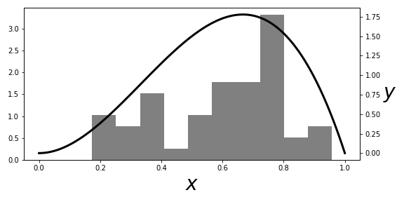
The $\beta(3,2)$ distribution and the # histogram that approximates it.
# #
#
#
#
# [Figure](#fig:Bootstrap_001) shows the
# $\beta(3,2)$ distribution and
# the corresponding histogram of the samples. The
# histogram represents
# $\hat{F}$ and is the distribution we sample from to obtain
# the
# bootstrap samples. As shown, the $\hat{F}$ is a pretty crude estimate
# for
# the $F$ density (smooth solid line), but that's not a serious
# problem insofar as
# the following bootstrap estimates are concerned.
# In fact, the approximation
# $\hat{F}$ has a naturally tendency to
# pull towards the bulk of probability mass.
# This is a
# feature, not a bug; and is the underlying mechanism that explains
# bootstrapping, but the formal proofs that exploit this basic
# idea are far out of
# our scope here. The next block generates the
# bootstrap samples
# In[5]:
yboot = np.random.choice(xsamples,(100,50))
yboot_mn = yboot.mean()
# and the bootstrap estimate is therefore,
# In[6]:
np.std(yboot.mean(axis=1)) # approx sqrt(1/1250)
# [Figure](#fig:Bootstrap_002) shows the distribution of computed
# sample means
# from the bootstrap samples. As promised, the next block
# shows how to use
# `sympy.stats` to compute the $\beta(3,2)$ parameters we quoted
# earlier.
# In[7]:
fig,ax = subplots()
fig.set_size_inches(8,4)
_=ax.hist(yboot.mean(axis=1),density=True,color='gray',rwidth=.8)
_=ax.set_title('Bootstrap std of sample mean %3.3f vs actual %3.3f'%
(np.std(yboot.mean(axis=1)),np.sqrt(1/1250.)))
fig.tight_layout()
fig.savefig('fig-statistics/Bootstrap_002.png')
#
#
#
#
#
#
#
#
#
# [Figure](#fig:Bootstrap_001) shows the
# $\beta(3,2)$ distribution and
# the corresponding histogram of the samples. The
# histogram represents
# $\hat{F}$ and is the distribution we sample from to obtain
# the
# bootstrap samples. As shown, the $\hat{F}$ is a pretty crude estimate
# for
# the $F$ density (smooth solid line), but that's not a serious
# problem insofar as
# the following bootstrap estimates are concerned.
# In fact, the approximation
# $\hat{F}$ has a naturally tendency to
# pull towards the bulk of probability mass.
# This is a
# feature, not a bug; and is the underlying mechanism that explains
# bootstrapping, but the formal proofs that exploit this basic
# idea are far out of
# our scope here. The next block generates the
# bootstrap samples
# In[5]:
yboot = np.random.choice(xsamples,(100,50))
yboot_mn = yboot.mean()
# and the bootstrap estimate is therefore,
# In[6]:
np.std(yboot.mean(axis=1)) # approx sqrt(1/1250)
# [Figure](#fig:Bootstrap_002) shows the distribution of computed
# sample means
# from the bootstrap samples. As promised, the next block
# shows how to use
# `sympy.stats` to compute the $\beta(3,2)$ parameters we quoted
# earlier.
# In[7]:
fig,ax = subplots()
fig.set_size_inches(8,4)
_=ax.hist(yboot.mean(axis=1),density=True,color='gray',rwidth=.8)
_=ax.set_title('Bootstrap std of sample mean %3.3f vs actual %3.3f'%
(np.std(yboot.mean(axis=1)),np.sqrt(1/1250.)))
fig.tight_layout()
fig.savefig('fig-statistics/Bootstrap_002.png')
#
#
#
#
# For each bootstrap draw, we compute the sample # mean. This is the histogram of those sample means that will be used to compute # the bootstrap estimate of the standard deviation.
# #
#
# In[8]:
import sympy as S
import sympy.stats
for i in range(50): # 50 samples
# load sympy.stats Beta random variables
# into global namespace using exec
execstring = "x%d = S.stats.Beta('x'+str(%d),3,2)"%(i,i)
exec(execstring)
# populate xlist with the sympy.stats random variables
# from above
xlist = [eval('x%d'%(i)) for i in range(50) ]
# compute sample mean
sample_mean = sum(xlist)/len(xlist)
# compute expectation of sample mean
sample_mean_1 = S.stats.E(sample_mean).evalf()
# compute 2nd moment of sample mean
sample_mean_2 = S.stats.E(S.expand(sample_mean**2)).evalf()
# standard deviation of sample mean
# use sympy sqrt function
sigma_smn = S.sqrt(sample_mean_2-sample_mean_1**2) # sqrt(2)/50
print(sigma_smn)
# **Programming Tip.**
#
# Using the `exec` function enables the creation of a
# sequence of Sympy
# random variables. Sympy has the `var` function which can
# automatically
# create a sequence of Sympy symbols, but there is no corresponding
# function in the statistics module to do this for random variables.
#
#
#
#
#
#
#
# **Example.** Recall the delta method
# from the section [sec:delta_method](#sec:delta_method). Suppose we have a set
# of Bernoulli coin-flips
# ($X_i$) with probability of head $p$. Our maximum
# likelihood estimator
# of $p$ is $\hat{p}=\sum X_i/n$ for $n$ flips. We know this
# estimator
# is unbiased with $\mathbb{E}(\hat{p})=p$ and $\mathbb{V}(\hat{p}) =
# p(1-p)/n$. Suppose we want to use the data to estimate the variance of
# the
# Bernoulli trials ($\mathbb{V}(X)=p(1-p)$). By the notation the
# delta method,
# $g(x) = x(1-x)$. By the plug-in principle, our maximum
# likelihood estimator of
# this variance is then $\hat{p}(1-\hat{p})$. We
# want the variance of this
# quantity. Using the results of the delta
# method, we have
#
# $$
# \begin{align*}
# \mathbb{V}(g(\hat{p})) &=(1-2\hat{p})^2\mathbb{V}(\hat{p})
# \\\
# \mathbb{V}(g(\hat{p})) &=(1-2\hat{p})^2\frac{\hat{p}(1-\hat{p})}{n} \\\
# \end{align*}
# $$
#
# Let's see how useful this is with a short simulation.
# In[9]:
import numpy as np
np.random.seed(123)
# In[10]:
from scipy import stats
import numpy as np
p= 0.25 # true head-up probability
x = stats.bernoulli(p).rvs(10)
print(x)
# The maximum likelihood estimator of $p$ is $\hat{p}=\sum X_i/n$,
# In[11]:
phat = x.mean()
print(phat)
# Then, plugging this into the delta method approximant above,
# In[12]:
print((1-2*phat)**2*(phat)**2/10)
# Now, let's try this using the bootstrap estimate of the variance
# In[13]:
phat_b=np.random.choice(x,(50,10)).mean(1)
print(np.var(phat_b*(1-phat_b)))
# This shows that the delta method's estimated variance
# is different from the
# bootstrap method, but which one is better?
# For this situation we can solve for
# this directly using Sympy
# In[14]:
import sympy as S
from sympy.stats import E, Bernoulli
xdata =[Bernoulli(i,p) for i in S.symbols('x:10')]
ph = sum(xdata)/float(len(xdata))
g = ph*(1-ph)
# **Programming Tip.**
#
# The argument in the `S.symbols('x:10')` function returns a
# sequence of Sympy
# symbols named `x1,x2` and so on. This is shorthand for
# creating and naming each
# symbol sequentially.
#
#
#
# Note that `g` is the
# $g(\hat{p})=\hat{p}(1- \hat{p})$
# whose variance we are trying to estimate.
# Then,
# we can plug in for the estimated $\hat{p}$ and get the correct
# value for
# the variance,
# In[15]:
print(E(g**2) - E(g)**2)
# This case is generally representative --- the delta method tends
# to
# underestimate the variance and the bootstrap estimate is better here.
#
#
# ## Parametric Bootstrap
#
# In the previous example, we used the $\lbrace x_1, x_2,
# \ldots, x_n \rbrace $
# samples themselves as the basis for $\hat{F}$ by weighting
# each with $1/n$. An
# alternative is to *assume* that the samples come from a
# particular
# distribution, estimate the parameters of that distribution from the
# sample set,
# and then use the bootstrap mechanism to draw samples from the
# assumed
# distribution, using the so-derived parameters. For example, the next
# code block
# does this for a normal distribution.
# In[19]:
n = 100
rv = stats.norm(0,2)
xsamples = rv.rvs(n)
# estimate mean and var from xsamples
mn_ = np.mean(xsamples)
std_ = np.std(xsamples)
# bootstrap from assumed normal distribution with
# mn_,std_ as parameters
rvb = stats.norm(mn_,std_) #plug-in distribution
yboot = rvb.rvs((n,500)).var(axis=0)
#
#
# Recall
# the sample variance estimator is the following:
#
# $$
# S^2 = \frac{1}{n-1} \sum (X_i-\bar{X})^2
# $$
#
# Assuming that the samples are normally distributed, this
# means that
# $(n-1)S^2/\sigma^2$ has a chi-squared distribution with
# $n-1$ degrees of
# freedom. Thus, the variance, $\mathbb{V}(S^2) = 2
# \sigma^4/(n-1) $. Likewise,
# the MLE plug-in estimate for this is
# $\mathbb{V}(S^2) = 2 \hat{\sigma}^4/(n-1)$
# The following code computes
# the variance of the sample variance, $S^2$ using the
# MLE and bootstrap
# methods.
# In[20]:
# MLE-Plugin Variance of the sample mean
print(2*std_**4/(n-1)) # MLE plugin
# Bootstrap variance of the sample mean
print(yboot.var())
# True variance of sample mean
print(2*(2**4)/(n-1))
#
#
# This
# shows that the bootstrap estimate is better here than the MLE
# plugin estimate.
# Note that this technique becomes even more powerful with multivariate
# distributions with many parameters because all the mechanics are the same.
# Thus,
# the bootstrap is a great all-purpose method for computing standard
# errors, but,
# in the limit, is it converging to the correct value? This is the
# question of
# *consistency*. Unfortunately, to answer this question requires more
# and deeper
# mathematics than we can get into here. The short answer is that for
# estimating
# standard errors, the bootstrap is a consistent estimator in a wide
# range of
# cases and so it definitely belongs in your toolkit.
#
#
# In[8]:
import sympy as S
import sympy.stats
for i in range(50): # 50 samples
# load sympy.stats Beta random variables
# into global namespace using exec
execstring = "x%d = S.stats.Beta('x'+str(%d),3,2)"%(i,i)
exec(execstring)
# populate xlist with the sympy.stats random variables
# from above
xlist = [eval('x%d'%(i)) for i in range(50) ]
# compute sample mean
sample_mean = sum(xlist)/len(xlist)
# compute expectation of sample mean
sample_mean_1 = S.stats.E(sample_mean).evalf()
# compute 2nd moment of sample mean
sample_mean_2 = S.stats.E(S.expand(sample_mean**2)).evalf()
# standard deviation of sample mean
# use sympy sqrt function
sigma_smn = S.sqrt(sample_mean_2-sample_mean_1**2) # sqrt(2)/50
print(sigma_smn)
# **Programming Tip.**
#
# Using the `exec` function enables the creation of a
# sequence of Sympy
# random variables. Sympy has the `var` function which can
# automatically
# create a sequence of Sympy symbols, but there is no corresponding
# function in the statistics module to do this for random variables.
#
#
#
#
#
#
#
# **Example.** Recall the delta method
# from the section [sec:delta_method](#sec:delta_method). Suppose we have a set
# of Bernoulli coin-flips
# ($X_i$) with probability of head $p$. Our maximum
# likelihood estimator
# of $p$ is $\hat{p}=\sum X_i/n$ for $n$ flips. We know this
# estimator
# is unbiased with $\mathbb{E}(\hat{p})=p$ and $\mathbb{V}(\hat{p}) =
# p(1-p)/n$. Suppose we want to use the data to estimate the variance of
# the
# Bernoulli trials ($\mathbb{V}(X)=p(1-p)$). By the notation the
# delta method,
# $g(x) = x(1-x)$. By the plug-in principle, our maximum
# likelihood estimator of
# this variance is then $\hat{p}(1-\hat{p})$. We
# want the variance of this
# quantity. Using the results of the delta
# method, we have
#
# $$
# \begin{align*}
# \mathbb{V}(g(\hat{p})) &=(1-2\hat{p})^2\mathbb{V}(\hat{p})
# \\\
# \mathbb{V}(g(\hat{p})) &=(1-2\hat{p})^2\frac{\hat{p}(1-\hat{p})}{n} \\\
# \end{align*}
# $$
#
# Let's see how useful this is with a short simulation.
# In[9]:
import numpy as np
np.random.seed(123)
# In[10]:
from scipy import stats
import numpy as np
p= 0.25 # true head-up probability
x = stats.bernoulli(p).rvs(10)
print(x)
# The maximum likelihood estimator of $p$ is $\hat{p}=\sum X_i/n$,
# In[11]:
phat = x.mean()
print(phat)
# Then, plugging this into the delta method approximant above,
# In[12]:
print((1-2*phat)**2*(phat)**2/10)
# Now, let's try this using the bootstrap estimate of the variance
# In[13]:
phat_b=np.random.choice(x,(50,10)).mean(1)
print(np.var(phat_b*(1-phat_b)))
# This shows that the delta method's estimated variance
# is different from the
# bootstrap method, but which one is better?
# For this situation we can solve for
# this directly using Sympy
# In[14]:
import sympy as S
from sympy.stats import E, Bernoulli
xdata =[Bernoulli(i,p) for i in S.symbols('x:10')]
ph = sum(xdata)/float(len(xdata))
g = ph*(1-ph)
# **Programming Tip.**
#
# The argument in the `S.symbols('x:10')` function returns a
# sequence of Sympy
# symbols named `x1,x2` and so on. This is shorthand for
# creating and naming each
# symbol sequentially.
#
#
#
# Note that `g` is the
# $g(\hat{p})=\hat{p}(1- \hat{p})$
# whose variance we are trying to estimate.
# Then,
# we can plug in for the estimated $\hat{p}$ and get the correct
# value for
# the variance,
# In[15]:
print(E(g**2) - E(g)**2)
# This case is generally representative --- the delta method tends
# to
# underestimate the variance and the bootstrap estimate is better here.
#
#
# ## Parametric Bootstrap
#
# In the previous example, we used the $\lbrace x_1, x_2,
# \ldots, x_n \rbrace $
# samples themselves as the basis for $\hat{F}$ by weighting
# each with $1/n$. An
# alternative is to *assume* that the samples come from a
# particular
# distribution, estimate the parameters of that distribution from the
# sample set,
# and then use the bootstrap mechanism to draw samples from the
# assumed
# distribution, using the so-derived parameters. For example, the next
# code block
# does this for a normal distribution.
# In[19]:
n = 100
rv = stats.norm(0,2)
xsamples = rv.rvs(n)
# estimate mean and var from xsamples
mn_ = np.mean(xsamples)
std_ = np.std(xsamples)
# bootstrap from assumed normal distribution with
# mn_,std_ as parameters
rvb = stats.norm(mn_,std_) #plug-in distribution
yboot = rvb.rvs((n,500)).var(axis=0)
#
#
# Recall
# the sample variance estimator is the following:
#
# $$
# S^2 = \frac{1}{n-1} \sum (X_i-\bar{X})^2
# $$
#
# Assuming that the samples are normally distributed, this
# means that
# $(n-1)S^2/\sigma^2$ has a chi-squared distribution with
# $n-1$ degrees of
# freedom. Thus, the variance, $\mathbb{V}(S^2) = 2
# \sigma^4/(n-1) $. Likewise,
# the MLE plug-in estimate for this is
# $\mathbb{V}(S^2) = 2 \hat{\sigma}^4/(n-1)$
# The following code computes
# the variance of the sample variance, $S^2$ using the
# MLE and bootstrap
# methods.
# In[20]:
# MLE-Plugin Variance of the sample mean
print(2*std_**4/(n-1)) # MLE plugin
# Bootstrap variance of the sample mean
print(yboot.var())
# True variance of sample mean
print(2*(2**4)/(n-1))
#
#
# This
# shows that the bootstrap estimate is better here than the MLE
# plugin estimate.
# Note that this technique becomes even more powerful with multivariate
# distributions with many parameters because all the mechanics are the same.
# Thus,
# the bootstrap is a great all-purpose method for computing standard
# errors, but,
# in the limit, is it converging to the correct value? This is the
# question of
# *consistency*. Unfortunately, to answer this question requires more
# and deeper
# mathematics than we can get into here. The short answer is that for
# estimating
# standard errors, the bootstrap is a consistent estimator in a wide
# range of
# cases and so it definitely belongs in your toolkit.